import pandas as pd
import numpy as np

url = 'http://archive.ics.uci.edu/ml/machine-learning-databases/horse-colic/horse-colic.data'
df = pd.read_csv(url, delim_whitespace=True, header=None)
df = df.replace("?", np.NaN)

df.fillna(0, inplace=True)
df.drop(columns=[2, 24, 25, 26, 27], inplace=True)
df[23].replace({1: 1, 2: 0}, inplace=True)
X = df.iloc[:, :-1].to_numpy().astype(float)
y = df[23].to_numpy().astype(int)

from sklearn.model_selection import train_test_split
X_train, X_test, y_train, y_test = train_test_split(X, y, test_size=0.15, random_state=42)

from sklearn.preprocessing import MinMaxScaler

mms = MinMaxScaler()
mms.fit(X_train)
X_train = mms.transform(X_train)
X_test = mms.transform(X_test)6 Netural networks
There are many different architects of netural networks. In our course we will only talk about the simplest one: multilayer perceptron (MLP). We will treat it as the generalization of logistic regression. In other words, we will treat logistic regression as an one-layer netural network. Under this idea, all the concepts and ideas, like gradient descent, mini-batch training, loss functions, learning curves, etc.. will be used.
6.1 Neural network: Back propagation
\[ \newcommand\diffp[2]{\dfrac{\partial #1}{\partial #2}} \]
To train a MLP model, we still use gradient descent. Therefore it is very important to know how to compute the gradient. Actually the idea is the same as logistic regreesion. The only issue is that now the model is more complicated. The gradient computation is summrized as an algorithm called back propagation. It is described as follows.
Here is an example of a Neural network with one hidden layer.
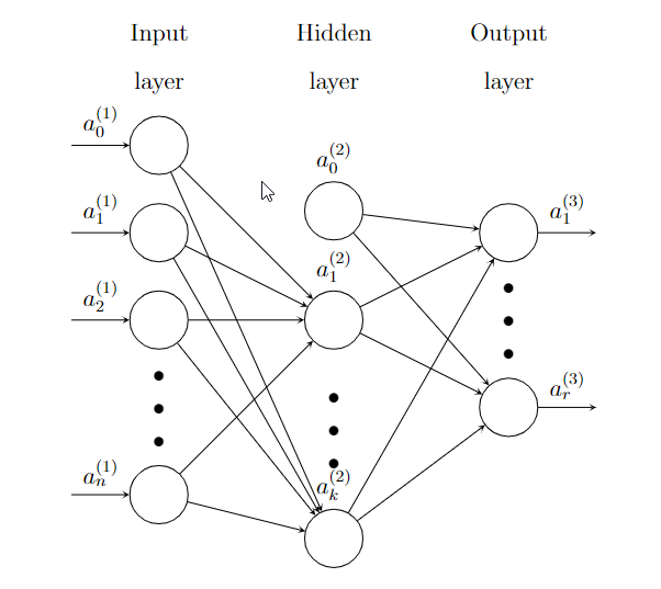
\(\Theta\) is the coefficients of the whole Neural network.
- \(a^{(1)}=\hat{\textbf{x}}\) is the input. \(a_0^{(1)}\) is added. This is an \((n+1)\)-dimension column vector.
- \(\Theta^{(1)}\) is the coefficient matrix from the input layer to the hidden layer, of size \(k\times(n+1)\).
- \(z^{(2)}=\Theta^{(1)}a^{(1)}\).
- \(a^{(2)}=\sigma(z^{(2)})\), and then add \(a^{(2)}_0\). This is an \((k+1)\)-dimension column vector.
- \(\Theta^{(2)}\) is the coefficient matrix from the hidden layer to the output layer, of size \(r\times(k+1)\).
- \(z^{(3)}=\Theta^{(2)}a^{(2)}\).
- \(a^{(3)}=\sigma(z^{(3)})\). Since this is the output layer, \(a^{(3)}_0\) won’t be added. % These \(a^{(3)}\) are \(h_{\Theta}(\textbf{x})\).
The dependency is as follows:
- \(J\) depends on \(z^{(3)}\) and \(a^{(3)}\).
- \(z^{(3)}\) and \(a^{(3)}\) depends on \(\Theta^{(2)}\) and \(a^{(2)}\).
- \(z^{(2)}\) and \(a^{(2)}\) depends on \(\Theta^{(1)}\) and \(a^{(1)}\).
- \(J\) depends on \(\Theta^{(1)}\), \(\Theta^{(2)}\) and \(a^{(1)}\).
Each layer is represented by the following diagram:
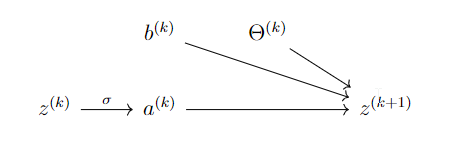
The diagram says:
\[ z^{(k+1)}=b^{(k)}+\Theta^{(k)}a^{(k)},\quad z^{(k+1)}_j=b^{(k)}_j+\sum \Theta^{(k)}_{jl}a^{(k)}_l,\quad a^{(k)}_j=\sigma(z^{(k)}_j). \]
Assume \(r,j\geq1\). Then
\[ \begin{aligned} \diffp{z^{(k+1)}_i}{a^{(k)}_r}&=\diffp*{\left(b^{(k)}_i+\sum\Theta^{(k)}_{il}a^{(k)}_l\right)}{a^{(k)}_r}=\Theta_{ir}^{(k)},\\ % \diffp{z^{(k+1)}_i}{\Theta^{(k)}_{ij}}&=\diffp*{\qty(a^{(k)}_0+\sum\Theta^{(k)}_{il}a^{(k)}_l)}{\Theta^{(k)}_{ij}}=a^{(k)}_j,\\ \diffp{z^{(k+1)}_i}{z^{(k)}_j}&=\sum_r \diffp{z^{(k+1)}_i}{a^{k}_r}\diffp{a^{(k)}_r}{z^{(k)}_j}+\sum_{p,g}\diffp{z^{(k+1)}_i}{\Theta^{(k)}_{pq}}\diffp{\Theta^{(k)}_{pq}}{z^{(k)}_j}+\sum_r \diffp{z^{(k+1)}_i}{b^{k}_r}\diffp{b^{(k)}_r}{z^{(k)}_j}\\ &=\sum_r \Theta^{(k)}_{ir}\diffp{a^{(k)}_r}{z^{(k)}_j}=\Theta^{(k)}_{ij}\diffp{a^{(k)}_j}{z^{(k)}_j}=\Theta^{(k)}_{ij}\sigma'(z^{(k)}_j),\\ \diffp{J}{z^{(k)}_j}&=\sum_r \diffp{J}{z^{(k+1)}_r}\diffp{z^{(k+1)}_r}{z^{(k)}_j}=\sum_r\diffp{J}{z^{(k+1)}_r}\Theta^{(k)}_{rj}\sigma'(z^{(k)}_j). \end{aligned} \]
We set
- \(\delta^k_j=\diffp{J}{z^{(k)}_j}\), \(\delta^k=\left[\delta^k_1,\delta_2^k,\ldots\right]^T\).
- \(\mathbf{z}^k=\left[z^{(k)}_1,z^{(k)}_2,\ldots\right]^T\), \(\mathbf{a}^k=\left[a^{(k)}_1,a^{(k)}_2,\ldots\right]^T\), \(\hat{\mathbf{a}}^k=\left[a^{(k)}_0,a^{(k)}_1,\ldots\right]^T\).
- \(\Theta^{k}=\left[\Theta^{(k)}_{ij}\right]\).
Then we have the following formula. Note that there are ``\(z_0\)’’ terms.
\[ \delta^k=\left[(\Theta^k)^T\delta^{k+1}\right]\circ \sigma'(\mathbf{z}^k). \]
\[ \begin{aligned} \diffp{z^{(k+1)}_r}{\Theta^{(k)}_{pq}}&=\diffp*{\left(b^{(k)}_r+\sum_l\Theta^{(k)}_{rl}a^{(k)}_l\right)}{\Theta^{(k)}_{pq}}=\begin{cases} 0&\text{ for }r\neq q,\\ a^{(k)}_q&\text{ for }r=q, \end{cases}\\ \diffp{J}{\Theta^{(k)}_{pq}}&=\sum_{r}\diffp{J}{z^{(k+1)}_r}\diffp{z^{(k+1)}_r}{\Theta^{(k)}_{pq}}=\diffp{J}{z^{(k+1)}_p}\diffp{z^{(k+1)}_p}{\Theta^{(k)}_{pq}}=\delta^{k+1}_pa^{k}_q,\\ \diffp{J}{b^{(k)}_{j}}&=\sum_{r}\diffp{J}{z^{(k+1)}_r}\diffp{z^{(k+1)}_r}{b^{(k)}_{j}}=\diffp{J}{z^{(k+1)}_j}\diffp{z^{(k+1)}_j}{b^{(k)}_{j}}=\diffp{J}{z^{(k+1)}_j}=\delta^{k+1}_j. \end{aligned} \]
Extend \(\hat{\Theta}=\left[b^{(k)},\Theta^{(k)}\right]\), and \(\partial^k J=\left[\diffp{J}{\hat{\Theta}^{(k)}_{ij}}\right]\). Then \[ \partial^k J=\left[\delta^{k+1}, \delta^{k+1}(\mathbf{a}^k)^T\right]. \] Then the algorithm is as follows.
- Starting from \(x\), \(y\) and some random \(\Theta\).
- Forward computation: compute \(z^{(k)}\) and \(a^{(k)}\). The last \(a^{(n)}\) is \(h\).
- Compute \(\delta^n=\nabla J\circ\sigma'(z^{(n)})\). In the case of \(J=\frac12||{h-y}||^2\), \(\nabla J=(a^{(n)}-y)\), and then \(\delta^n=(a^{(n)}-y)\circ\sigma'(z^{(n)})\).
- Backwards: \(\delta^k=\left[(\Theta^k)^T\delta^{k+1}\right]\circ \sigma'(\mathbf{z}^k)\), and \(\partial^k J=\left[\delta^{k+1}, \delta^{k+1}(\mathbf{a}^k)^T\right]\) .
Example 6.1 Consider there are 3 layers: input, hidden and output. There are \(m+1\) nodes in the input layer, \(n+1\) nodes in the hidden layer and \(k\) in the output layer. Therefore
- \(a^{(1)}\) and \(\delta^1\) are \(m\)-dim column vectors.
- \(z^{(2)}\), \(a^{(2)}\) and \(\delta^2\) are \(n\)-dim column vectors.
- \(z^{(3)}\), \(a^{(3)}\) and \(\delta^3\) are \(k\)-dim column vectors.
- \(\hat{\Theta}^1\) is \(n\times(m+1)\), \(\hat{\Theta}^2\) is \(k\times(n+1)\).
- \(z^{(2)}=b^{(1)}+\Theta^{(1)}a^{(1)}=\hat{\Theta}^{(1)}\hat{a}^{(1)}\), \(z^{(3)}=b^{(2)}+\Theta^{(2)}a^{(2)}=\hat{\Theta}^{(2)}\hat{a}^{(2)}\).
- \(\delta^3=\nabla_aJ\circ\sigma'(z^{(3)})\). This is a \(k\)-dim column vector.
- \(\partial^2 J=\left[\delta^3,\delta^3(a^{(2)})^T\right]\).
- \(\delta^2=\left[(\Theta^2)^T\delta^3\right]\circ \sigma'(z^{(2)})\), where \((\hat{\Theta^2})^T\delta^3=(\hat{\Theta^2})^T\delta^3\) and then remove the first row.
- \(\delta^1=\begin{bmatrix}(\Theta^1)^T\delta^2\end{bmatrix}\circ \sigma'(z^{(1)})\), where \((\hat{\Theta^1})^T\delta^2=(\hat{\Theta^1})^T\delta^2\) and then remove the first row.
- \(\partial^1 J=\left[\delta^2,\delta^2(a^{(1)})^T\right]\).
- When \(J=-\frac1m\sum y\ln a+(1-y)\ln(1-a)\), \(\delta^3=\frac1m(\sum a^{(3)}-\sum y)\).
6.2 Example
Let us take some of our old dataset as an example. This is an continuation of the horse colic dataset from Logistic regression.
Now we build a neural network. This is a 2-layer model, with 1 hidden layer with 10 nodes.
import keras_core as keras
from keras import models, layers, Input
model = models.Sequential()

model.add(Input(shape=(X_train.shape[1],)))
model.add(layers.Dense(10, activation='sigmoid'))
model.add(layers.Dense(1, activation='sigmoid'))

model.compile(optimizer='adam', loss='binary_crossentropy', metrics=['accuracy'])
hist = model.fit(X_train, y_train, epochs=500, batch_size=30, validation_data=(X_test, y_test), verbose=0)

loss_train = hist.history['loss']
loss_val = hist.history['val_loss']

acc_train = hist.history['accuracy']
acc_val = hist.history['val_accuracy']
And the learning curve are shown in the following plots.
import matplotlib.pyplot as plt
fig, ax = plt.subplots(1, 2)
ax[0].plot(loss_train, label='train_loss')
ax[0].plot(loss_val, label='val_loss')
ax[0].legend()

ax[1].plot(acc_train, label='train_acc')
ax[1].plot(acc_val, label='val_acc')
ax[1].legend()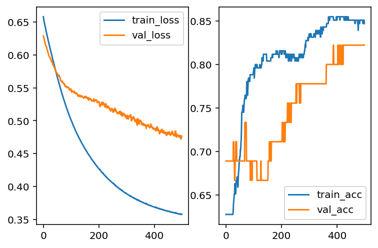
It seems that our model has overfitting issues. Therefore we need to modifify the architects of our model. The first idea is to add L2 regularization as we talked about it in LogsiticRegression case. Here we use 0.01 as the regularization strenth.
Let us add the layer to the model and retrain it.
import keras_core as keras
from keras import regularizers
model = models.Sequential()

model.add(layers.Dense(10, activation='sigmoid', input_dim=X_train.shape[1], kernel_regularizer=regularizers.l2(0.01)))
model.add(layers.Dense(1, activation='sigmoid', kernel_regularizer=regularizers.l2(0.01)))

model.compile(optimizer='adam', loss='binary_crossentropy', metrics=['accuracy'])
hist = model.fit(X_train, y_train, epochs=500, batch_size=30, validation_data=(X_test, y_test), verbose=0)

loss_train = hist.history['loss']
loss_val = hist.history['val_loss']

acc_train = hist.history['accuracy']
acc_val = hist.history['val_accuracy']
import matplotlib.pyplot as plt
fig, ax = plt.subplots(1, 2)
ax[0].plot(loss_train, label='train_loss')
ax[0].plot(loss_val, label='val_loss')
ax[0].legend()
ax[1].plot(acc_train, label='train_acc')
ax[1].plot(acc_val, label='val_acc')
ax[1].legend()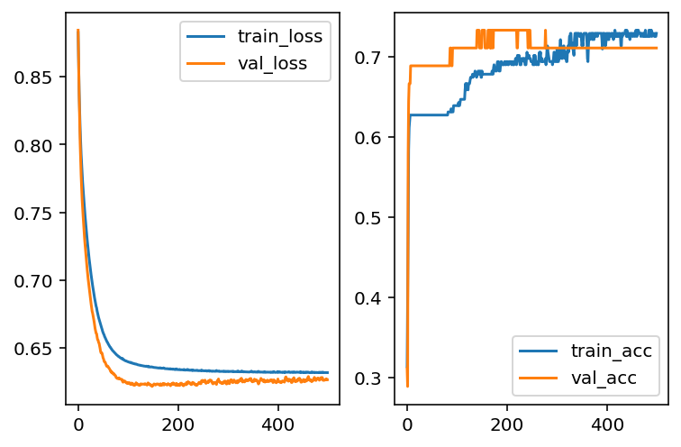
Another way to deal with overfitting is to add a Dropout layer. The idea is that when training the model, part of the data will be randomly discarded. Then after fitting, the model tends to reduce the variance, and then reduce the overfitting.
The code of a Dropout layer is listed below. Note that the number represents the percentage of the training data that will be dropped.
import keras_core as keras
from keras import regularizers
model = models.Sequential()

model.add(layers.Dense(10, activation='sigmoid', input_dim=X_train.shape[1]))
model.add(layers.Dropout(0.3))
model.add(layers.Dense(1, activation='sigmoid'))

model.compile(optimizer='adam', loss='binary_crossentropy', metrics=['accuracy'])
hist = model.fit(X_train, y_train, epochs=500, batch_size=30, validation_data=(X_test, y_test), verbose=0)

loss_train = hist.history['loss']
loss_val = hist.history['val_loss']

acc_train = hist.history['accuracy']
acc_val = hist.history['val_accuracy']
import matplotlib.pyplot as plt
fig, ax = plt.subplots(1, 2)
ax[0].plot(loss_train, label='train_loss')
ax[0].plot(loss_val, label='val_loss')
ax[0].legend()
ax[1].plot(acc_train, label='train_acc')
ax[1].plot(acc_val, label='val_acc')
ax[1].legend()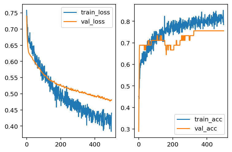
After playing with different hyperparameters, the overfitting issues seem to be better (but not entirely fixed). However, the overall performance is getting worse. This means that the model is moving towards underfitting side. Then we may add more layers to make the model more complicated in order to capture more information.
import keras_core as keras
from keras import regularizers
model = models.Sequential()

model.add(layers.Dense(10, activation='sigmoid', input_dim=X_train.shape[1]))
model.add(layers.Dropout(0.3))
model.add(layers.Dense(10, activation='sigmoid', input_dim=X_train.shape[1]))
model.add(layers.Dropout(0.1))
model.add(layers.Dense(1, activation='sigmoid'))

model.compile(optimizer='adam', loss='binary_crossentropy', metrics=['accuracy'])
hist = model.fit(X_train, y_train, epochs=500, batch_size=30, validation_data=(X_test, y_test), verbose=0)

loss_train = hist.history['loss']
loss_val = hist.history['val_loss']

acc_train = hist.history['accuracy']
acc_val = hist.history['val_accuracy']
import matplotlib.pyplot as plt
fig, ax = plt.subplots(1, 2)
ax[0].plot(loss_train, label='train_loss')
ax[0].plot(loss_val, label='val_loss')
ax[0].legend()
ax[1].plot(acc_train, label='train_acc')
ax[1].plot(acc_val, label='val_acc')
ax[1].legend()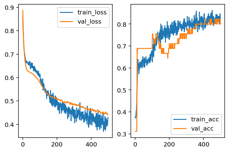
As you may see, to build a netural network model it requires many testing. There are many established models. When you build your own architecture, you may start from there and modify it to fit your data.
6.3 Exercises and Projects
Exercise 6.1 Please hand write a report about the details of back propagation.
Exercise 6.2 CHOOSE ONE: Please use netural network to one of the following datasets. - the iris dataset. - the dating dataset. - the titanic dataset.
Please in addition answer the following questions.
- What is your accuracy score?
- How many epochs do you use?
- What is the batch size do you use?
- Plot the learning curve (loss vs epochs, accuracy vs epochs).
- Analyze the bias / variance status.