10 Projects with R

10.1 WHO TB dataset

Let us explore the tuberculosis cases data. The dataset is provided by WHO and can be downloaded from here. tidyr also provides the dataset. You may directly get the dataset after you load tidyr from tidyverse. The variable description can be found from tidyr documentations.

library(tidyverse)
#> ── Attaching core tidyverse packages ──────────────────────── tidyverse 2.0.0 ──
#> ✔ dplyr     1.1.1     ✔ readr     2.1.4
#> ✔ forcats   1.0.0     ✔ stringr   1.5.0
#> ✔ ggplot2   3.4.2     ✔ tibble    3.2.1
#> ✔ lubridate 1.9.2     ✔ tidyr     1.3.0
#> ✔ purrr     1.0.1     
#> ── Conflicts ────────────────────────────────────────── tidyverse_conflicts() ──
#> ✖ dplyr::filter() masks stats::filter()
#> ✖ dplyr::lag()    masks stats::lag()
#> ℹ Use the conflicted package (<http://conflicted.r-lib.org/>) to force all conflicts to become errors
who
#> # A tibble: 7,240 × 60
#>    country  iso2  iso3   year new_sp_m014 new_sp_m1524 new_sp_m2534 new_sp_m3544
#>    <chr>    <chr> <chr> <dbl>       <dbl>        <dbl>        <dbl>        <dbl>
#>  1 Afghani… AF    AFG    1980          NA           NA           NA           NA
#>  2 Afghani… AF    AFG    1981          NA           NA           NA           NA
#>  3 Afghani… AF    AFG    1982          NA           NA           NA           NA
#>  4 Afghani… AF    AFG    1983          NA           NA           NA           NA
#>  5 Afghani… AF    AFG    1984          NA           NA           NA           NA
#>  6 Afghani… AF    AFG    1985          NA           NA           NA           NA
#>  7 Afghani… AF    AFG    1986          NA           NA           NA           NA
#>  8 Afghani… AF    AFG    1987          NA           NA           NA           NA
#>  9 Afghani… AF    AFG    1988          NA           NA           NA           NA
#> 10 Afghani… AF    AFG    1989          NA           NA           NA           NA
#> # ℹ 7,230 more rows
#> # ℹ 52 more variables: new_sp_m4554 <dbl>, new_sp_m5564 <dbl>,
#> #   new_sp_m65 <dbl>, new_sp_f014 <dbl>, new_sp_f1524 <dbl>,
#> #   new_sp_f2534 <dbl>, new_sp_f3544 <dbl>, new_sp_f4554 <dbl>,
#> #   new_sp_f5564 <dbl>, new_sp_f65 <dbl>, new_sn_m014 <dbl>,
#> #   new_sn_m1524 <dbl>, new_sn_m2534 <dbl>, new_sn_m3544 <dbl>,
#> #   new_sn_m4554 <dbl>, new_sn_m5564 <dbl>, new_sn_m65 <dbl>, …

Based on the description of varaibles, we understand that

country, iso2, iso3 are all refered to country names (and thus they are redundant).
Columns after year, like new_sp_m014 etc., are counts of new TB cases recorded by groups. The code has three parts, most of which are separated by _ (but there are some exceptions).
- The first part is always new.
- The second part is a code for method of diagnosis:
  - rel = relapse,
  - sn = negative pulmonary smear,
  - sp = positive pulmonary smear,
  - ep = extrapulmonary.
- The third part is a code for gender (f = female, m = male) and a code for age group:
  - 014 = 0-14 yrs of age,
  - 1524 = 15-24 years of age,
  - 2534 = 25 to 34 years of age,
  - 3544 = 35 to 44 years of age,
  - 4554 = 45 to 54 years of age,
  - 5564 = 55 to 64 years of age,
  - 65 = 65 years of age or older

Therefore to clean the data, we need the following steps.

Example 10.1 Gather together all the columns from new_sp_m014 to newrel_f65.

Tip

wholonger <- who %>% pivot_longer(cols=5:60, names_to='group', values_to='counts')

Then we use stringr::str_replace() to replace newrel by new_rel.

wholonger2 <- wholonger %>% mutate(key=str_replace(group, 'newrel', 'new_rel'))

Example 10.2 Parse the column group into columns.

Tip

wholonger3 <- wholonger2 %>% 
        separate(key, into=c('new', 'type', 'genderage'), sep='_') %>% 
        separate(genderage, into=c('gender', 'age'), sep=1)

Example 10.3 Pick the columns that matters.

Tip

tidywho <- wholonger3[c('country', 'year', 'type', 'gender', 'age', 'counts')]

We could use the pipe symbol to connect all the above steps.

Tip

tidywho <- who %>% 
    pivot_longer(cols=5:60, names_to='group', values_to='counts') %>% 
    mutate(key=str_replace(group, 'newrel', 'new_rel')) %>% 
    separate(key, into=c('new', 'type', 'genderage'), sep='_') %>% 
    separate(genderage, into=c('gender', 'age'), sep=1) %>% 
    select('country', 'year', 'type', 'gender', 'age', 'counts')

10.2 US Babynames

Let us use R to solve the babynames dataset again.

The first task is to read those files.

Example 10.4 Please read files and put the data into one tibble. The dataset can be downloaded from here as a zip file.

Tip

path <- 'assessts/datasets/babynames/yob'
dfs <- map(1880:2010, function(y){
    filepath <- paste0(path, as.character(y), '.txt')
    df_individual <- tibble(read.csv(filepath, header=FALSE))
    names(df_individual) <- c('name', 'gender', 'counts')
    df_individual$year <- y
    df_individual
})
df <- bind_rows(dfs)

Example 10.5 Please plot the total births by gender and year.

Tip

df %>% 
    group_by(gender, year) %>% 
    summarize(total_num=sum(counts)) %>% 
    ggplot() +
        geom_line(mapping = aes(x=year, y=total_num, color=gender))
#> `summarise()` has grouped output by 'gender'. You can override using the
#> `.groups` argument.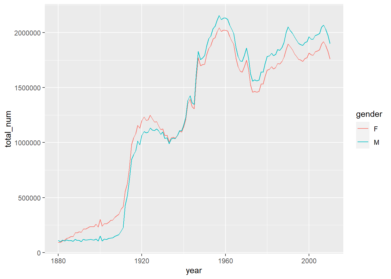

Example 10.6 Please compute the proportions of each name relateive to the total number of births per year per gender.

Tip

df %>% 
    group_by(gender, year) %>% 
    mutate(prop=counts/sum(counts))
#> # A tibble: 1,690,784 × 5
#> # Groups:   gender, year [262]
#>    name      gender counts  year   prop
#>    <chr>     <chr>   <int> <int>  <dbl>
#>  1 Mary      F        7065  1880 0.0776
#>  2 Anna      F        2604  1880 0.0286
#>  3 Emma      F        2003  1880 0.0220
#>  4 Elizabeth F        1939  1880 0.0213
#>  5 Minnie    F        1746  1880 0.0192
#>  6 Margaret  F        1578  1880 0.0173
#>  7 Ida       F        1472  1880 0.0162
#>  8 Alice     F        1414  1880 0.0155
#>  9 Bertha    F        1320  1880 0.0145
#> 10 Sarah     F        1288  1880 0.0142
#> # ℹ 1,690,774 more rows

Example 10.7 We would like to keep the first 100 names (by counts) in each year and save it as a new tibble top100.

Tip

top100 <- df %>% 
        group_by(gender, year) %>% 
        top_n(100, wt=counts)

Example 10.8 Please draw the trend of John, Harry, Mary in top100 by counts.

Tip

namelist <- c('John', 'Harry', 'Mary')
top100 %>% 
    filter(name %in% namelist) %>% 
    ggplot() +
        geom_line(mapping=aes(x=year, y=counts, color=name))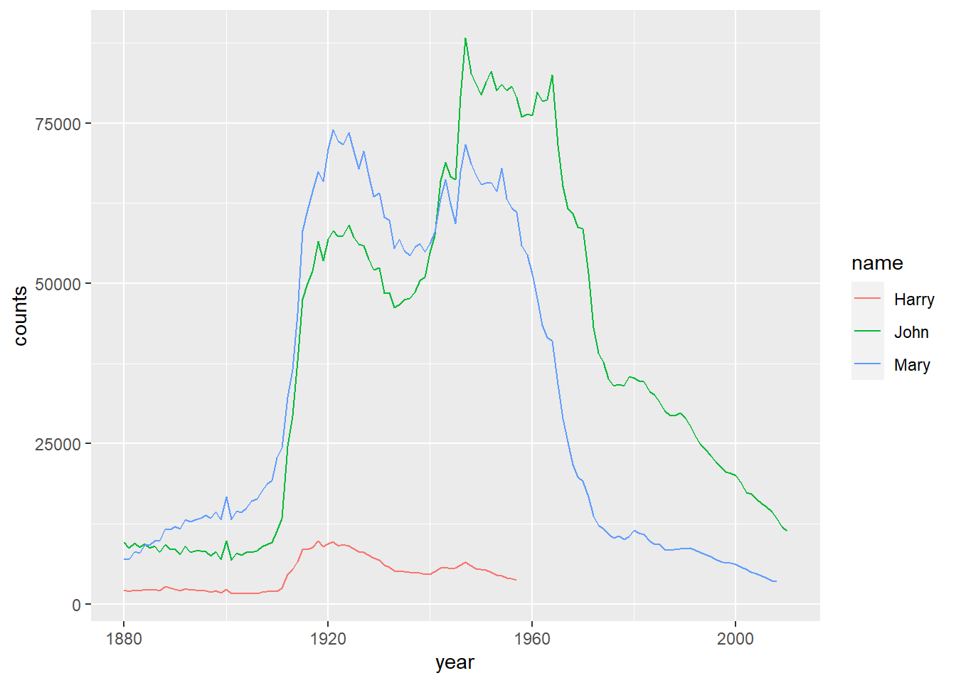

Example 10.9 Now we would like to analyze the ending of names. Please get a tibble that contains the counts of ending letter per year per gender. We mainly focus on 1910, 1960 and 2010.

Tip

df %>% 
    filter(year %in% c(1910, 1960, 2010)) %>% 
    mutate(ending=str_sub(name, -1, -1), 
           year=as.factor(year)) %>% 
    group_by(gender, year, ending) %>% 
    summarise(ending_counts=sum(counts)) %>% 
    ggplot() +
        geom_col(
            mapping = aes(
                x=ending, 
                y=ending_counts, 
                fill=year,
                ), 
            position = "dodge",
        ) +
        facet_wrap(~gender, nrow=2)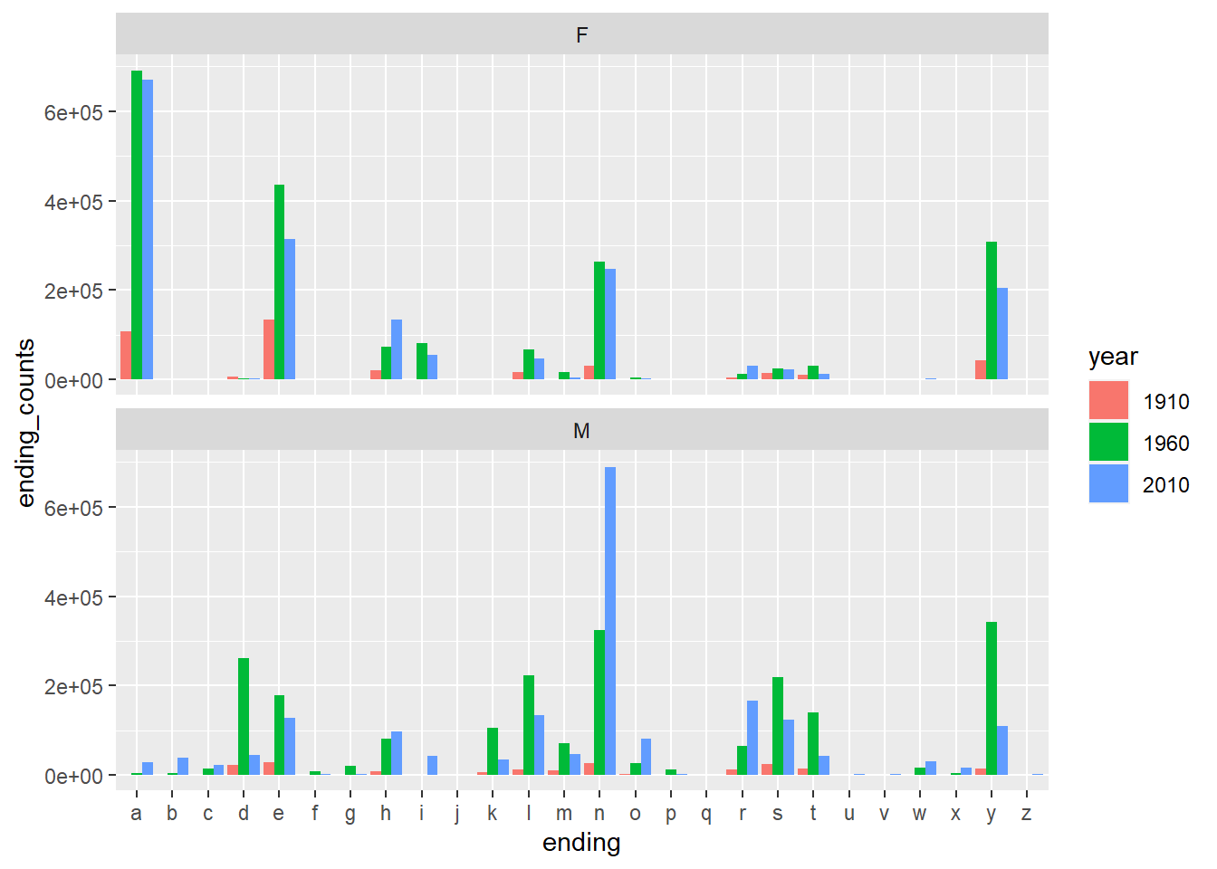

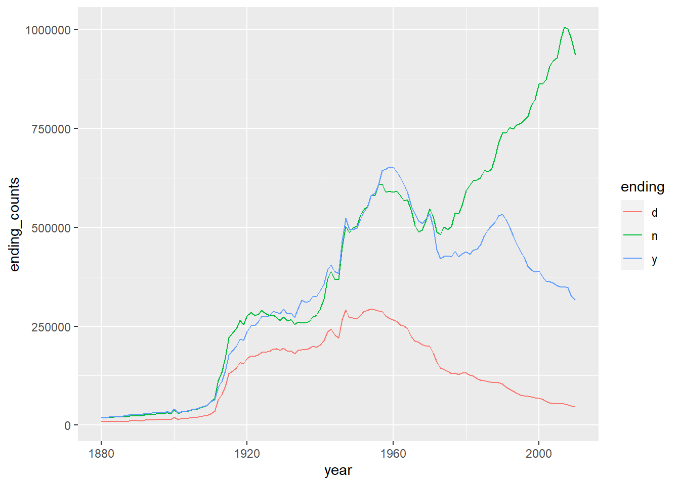
Example 10.10 Please draw the line plot to show the trending of certain letters through years. Here we choose d, n and y.

Tip

df %>% 
    mutate(ending=str_sub(name, -1, -1)) %>% 
    group_by(year, ending) %>% 
    summarise(ending_counts=sum(counts)) %>% 
    filter(ending %in% c('d', 'n', 'y')) %>% 
    ggplot() +
        geom_line(
            mapping = aes(
                x=year, 
                y=ending_counts, 
                color=ending
            )
        )

10.1 WHO TB dataset

10.2 US Babynames

References