9 R for Data Sciences

The main reference for this Chapter is [1].

9.1 `tibble`

tidyverse mainly deals with tibble instead of data.frame. Therefore this is where we start.

tibble is a data.frame with different attributes and requirements. The package tibble provides support for tibble. It is included in tidyverse. To load it, you just use the code:

library(tidyverse)
#> ── Attaching core tidyverse packages ──────────────────────── tidyverse 2.0.0 ──
#> ✔ dplyr     1.1.1     ✔ readr     2.1.4
#> ✔ forcats   1.0.0     ✔ stringr   1.5.0
#> ✔ ggplot2   3.4.2     ✔ tibble    3.2.1
#> ✔ lubridate 1.9.2     ✔ tidyr     1.3.0
#> ✔ purrr     1.0.1     
#> ── Conflicts ────────────────────────────────────────── tidyverse_conflicts() ──
#> ✖ dplyr::filter() masks stats::filter()
#> ✖ dplyr::lag()    masks stats::lag()
#> ℹ Use the conflicted package (<http://conflicted.r-lib.org/>) to force all conflicts to become errors

9.1.1 Create tibbles

Here is an example of creating tibbles.

Example 9.1

tbl <- tibble(x=1:5, y=1, z=x^2+y)
tbl
#> # A tibble: 5 × 3
#>       x     y     z
#>   <int> <dbl> <dbl>
#> 1     1     1     2
#> 2     2     1     5
#> 3     3     1    10
#> 4     4     1    17
#> 5     5     1    26
attributes(tbl)
#> $class
#> [1] "tbl_df"     "tbl"        "data.frame"
#> 
#> $row.names
#> [1] 1 2 3 4 5
#> 
#> $names
#> [1] "x" "y" "z"

Note that it is more flexible to create a tibble since tibble() will automatically recycle inputs and allows you to refer to variables that you just created.

Note

In the past (for a very long time), when using data.frame() to create a data.frame, it will automatically convert strings to factors. This is changed recently that the default setting is not to convert.

When using tibble() to create a tibble, the type of the inputs will never be changed.

Note

In tibble you may use nonsyntactic names as column names, which are invalid R variable names. To refer to these variables, you need to surround them with backticks `.

tb <- tibble(
    `:)` = "smile",
    ` ` = "space",
    `2000` = "number"
)
tb
#> # A tibble: 1 × 3
#>   `:)`  ` `   `2000`
#>   <chr> <chr> <chr> 
#> 1 smile space number

9.1.2 Differences between tibble and data.frame.

9.1.2.1 Printing

Tibbles have a refined print method that shows only the first 10 rows and all the columns that fit on screen.

deck <- tibble(suit=rep(c('spades', 'hearts', 'clubs', 'diamonds'), 13), face=rep(1:13, 4))
deck
#> # A tibble: 52 × 2
#>    suit      face
#>    <chr>    <int>
#>  1 spades       1
#>  2 hearts       2
#>  3 clubs        3
#>  4 diamonds     4
#>  5 spades       5
#>  6 hearts       6
#>  7 clubs        7
#>  8 diamonds     8
#>  9 spades       9
#> 10 hearts      10
#> # ℹ 42 more rows

9.1.2.2 Subsetting

To get a single value, [[]] or $ should be used, just like for data.frame. These two are almost the same. The only difference is that [[]] accepts positions, but $ only accepts names.

To be used in a pipe, the special placeholder . will be used.

deck %>% .$face
#>  [1]  1  2  3  4  5  6  7  8  9 10 11 12 13  1  2  3  4  5  6  7  8  9 10 11 12
#> [26] 13  1  2  3  4  5  6  7  8  9 10 11 12 13  1  2  3  4  5  6  7  8  9 10 11
#> [51] 12 13

We will talk about pipes later.

9.1.3 `%>%` symbol

%>% is the pipeline symbol, which is another way to connect several functions. Most functions in tidyverse have the first argument data, and both the input data and the output are tibbles. The syntax here is that data %>% function(arguments) is the same as function(data, arguments). The benefit is that it is easier to have many functions consecutively applied to the data. Please see the following example.

data %>% function1(arguments1)
    %>% function2(arguments2)
    %>% function3(arguments3)
    %>% function4(arguments4)

function4(function3(function2(function1(data, arguments1), arguments2), arguments3), arguments4)

data2 <- function1(data, arguments1)
data3 <- function2(data2, arguments2)
data4 <- function3(data3, arguments3)
function4(data4, arguments4)

The readability of the first one is much better than the second one. Comparing to the third one, we don’t need to create a lot of intermedia temporary variables.

9.2 Tidy Data

The same underlying data can be represented in multiple ways. The following example shows the same data organized in four different ways.

Example 9.2 These tibbles are provided by tidyr. You could directly load it from tidyverse.

library(tidyverse)
data(table1, package='tidyr')
data(table2, package='tidyr')
data(table3, package='tidyr')
data(table4a, package='tidyr')
data(table4b, package='tidyr')

table1

table1
#> # A tibble: 6 × 4
#>   country      year  cases population
#>   <chr>       <dbl>  <dbl>      <dbl>
#> 1 Afghanistan  1999    745   19987071
#> 2 Afghanistan  2000   2666   20595360
#> 3 Brazil       1999  37737  172006362
#> 4 Brazil       2000  80488  174504898
#> 5 China        1999 212258 1272915272
#> 6 China        2000 213766 1280428583

table2

table2
#> # A tibble: 12 × 4
#>    country      year type            count
#>    <chr>       <dbl> <chr>           <dbl>
#>  1 Afghanistan  1999 cases             745
#>  2 Afghanistan  1999 population   19987071
#>  3 Afghanistan  2000 cases            2666
#>  4 Afghanistan  2000 population   20595360
#>  5 Brazil       1999 cases           37737
#>  6 Brazil       1999 population  172006362
#>  7 Brazil       2000 cases           80488
#>  8 Brazil       2000 population  174504898
#>  9 China        1999 cases          212258
#> 10 China        1999 population 1272915272
#> 11 China        2000 cases          213766
#> 12 China        2000 population 1280428583

table3

table3
#> # A tibble: 6 × 3
#>   country      year rate             
#>   <chr>       <dbl> <chr>            
#> 1 Afghanistan  1999 745/19987071     
#> 2 Afghanistan  2000 2666/20595360    
#> 3 Brazil       1999 37737/172006362  
#> 4 Brazil       2000 80488/174504898  
#> 5 China        1999 212258/1272915272
#> 6 China        2000 213766/1280428583

Spread across two tibbles.

table4a
#> # A tibble: 3 × 3
#>   country     `1999` `2000`
#>   <chr>        <dbl>  <dbl>
#> 1 Afghanistan    745   2666
#> 2 Brazil       37737  80488
#> 3 China       212258 213766

table4b
#> # A tibble: 3 × 3
#>   country         `1999`     `2000`
#>   <chr>            <dbl>      <dbl>
#> 1 Afghanistan   19987071   20595360
#> 2 Brazil       172006362  174504898
#> 3 China       1272915272 1280428583

Definition 9.1 A dataset is tidy if

Each variable have its own column.
Each observation have its own row.
Each value have its oven cell.

These three conditions are interrelated because it is impossible to only satisfy two of the three. In pratical, we need to follow the instructions:

Put each dataset in a tibble.
Put each variable in a column.

Tidy data is a consistent way to organize your data in R. The main advantages are:

It is one consistent way of storing data. In other words, this is a consistent data structure that can be used in many cases.
To placing variables in columns allows R’s vectorized nature to shine.

All packages in the tidyverse are designed to work with tidy data.

9.2.1 Tidying datasets

Most datasets are untidy:

One variable might be spread across multiple columns.
One observation might be scattered across multiple rows.

9.2.1.1 `pivot_longer()`

A common problem is that the column names are not names of variables, but values of a variable. For example, table4a above has columns 1999 and 2000. These two names are actually the values of a variable year. In addition, each row represents two observations, not one.

table4a
#> # A tibble: 3 × 3
#>   country     `1999` `2000`
#>   <chr>        <dbl>  <dbl>
#> 1 Afghanistan    745   2666
#> 2 Brazil       37737  80488
#> 3 China       212258 213766

To tidy this type of dataset, we need to gather those columns into a new pair of variables. We need three parameters:

The set of columns that represent values. In this case, those are 1999 and 2000.
The name of the variable. In this case, it is year. -The name of the variable whose values are spread over the cells. In this case, it is the number of cases.

Then we apply pivot_longer().

pivot_longer(table4a, cols=c(`1999`, `2000`), names_to='year', values_to='cases')
#> # A tibble: 6 × 3
#>   country     year   cases
#>   <chr>       <chr>  <dbl>
#> 1 Afghanistan 1999     745
#> 2 Afghanistan 2000    2666
#> 3 Brazil      1999   37737
#> 4 Brazil      2000   80488
#> 5 China       1999  212258
#> 6 China       2000  213766

We may also use the pipe %>% symbol.

table4a %>% pivot_longer(cols=c(`1999`, `2000`), names_to='year', values_to='cases')
#> # A tibble: 6 × 3
#>   country     year   cases
#>   <chr>       <chr>  <dbl>
#> 1 Afghanistan 1999     745
#> 2 Afghanistan 2000    2666
#> 3 Brazil      1999   37737
#> 4 Brazil      2000   80488
#> 5 China       1999  212258
#> 6 China       2000  213766

We can do the similar thing to table4b. Then we could combine the two tibbles together.

tidy4a <- table4a %>% 
    pivot_longer(cols=c(`1999`, `2000`), names_to='year', values_to='cases')
tidy4b <- table4b %>% 
    pivot_longer(cols=c(`1999`, `2000`), names_to='year', values_to='population')
left_join(tidy4a, tidy4b)
#> Joining with `by = join_by(country, year)`
#> # A tibble: 6 × 4
#>   country     year   cases population
#>   <chr>       <chr>  <dbl>      <dbl>
#> 1 Afghanistan 1999     745   19987071
#> 2 Afghanistan 2000    2666   20595360
#> 3 Brazil      1999   37737  172006362
#> 4 Brazil      2000   80488  174504898
#> 5 China       1999  212258 1272915272
#> 6 China       2000  213766 1280428583

pivot_longer() is an updated approach to gather(), designed to be both simpler to use and to handle more use cases. We recommend you use pivot_longer() for new code; gather() isn’t going away but is no longer under active development.

9.2.1.2 `pivot_wider()`

Another issuse is that an observation is scattered across multiple rows. Take table2 as an example. An observation is a country in a year, but each observation is spread across two rows.

table2
#> # A tibble: 12 × 4
#>    country      year type            count
#>    <chr>       <dbl> <chr>           <dbl>
#>  1 Afghanistan  1999 cases             745
#>  2 Afghanistan  1999 population   19987071
#>  3 Afghanistan  2000 cases            2666
#>  4 Afghanistan  2000 population   20595360
#>  5 Brazil       1999 cases           37737
#>  6 Brazil       1999 population  172006362
#>  7 Brazil       2000 cases           80488
#>  8 Brazil       2000 population  174504898
#>  9 China        1999 cases          212258
#> 10 China        1999 population 1272915272
#> 11 China        2000 cases          213766
#> 12 China        2000 population 1280428583

We could apply pivot_wider() to make it tidy. Here we need two arguments.

The column that contains variable names. Here, it’s type.
The column that contains values forms multiple variables. Here, it’s count.

pivot_wider(table2, names_from='type', values_from='count')
#> # A tibble: 6 × 4
#>   country      year  cases population
#>   <chr>       <dbl>  <dbl>      <dbl>
#> 1 Afghanistan  1999    745   19987071
#> 2 Afghanistan  2000   2666   20595360
#> 3 Brazil       1999  37737  172006362
#> 4 Brazil       2000  80488  174504898
#> 5 China        1999 212258 1272915272
#> 6 China        2000 213766 1280428583

We can also use the pipe symbol %>%.

table2 %>% pivot_wider(names_from='type', values_from='count')
#> # A tibble: 6 × 4
#>   country      year  cases population
#>   <chr>       <dbl>  <dbl>      <dbl>
#> 1 Afghanistan  1999    745   19987071
#> 2 Afghanistan  2000   2666   20595360
#> 3 Brazil       1999  37737  172006362
#> 4 Brazil       2000  80488  174504898
#> 5 China        1999 212258 1272915272
#> 6 China        2000 213766 1280428583

pivot_wider() is an updated approach to spread(), designed to be both simpler to use and to handle more use cases. We recommend you use pivot_wider() for new code; spread() isn’t going away but is no longer under active development.

9.2.1.3 `separate()`

If we would like to split one columns into multiple columns since there are more than one values in a cell, we could use separate().

separate(table3, rate, into=c('cases', 'population'))
#> # A tibble: 6 × 4
#>   country      year cases  population
#>   <chr>       <dbl> <chr>  <chr>     
#> 1 Afghanistan  1999 745    19987071  
#> 2 Afghanistan  2000 2666   20595360  
#> 3 Brazil       1999 37737  172006362 
#> 4 Brazil       2000 80488  174504898 
#> 5 China        1999 212258 1272915272
#> 6 China        2000 213766 1280428583

We could also use the pipe symbol %>%.

table3 %>% separate(rate, into=c('cases', 'population'))
#> # A tibble: 6 × 4
#>   country      year cases  population
#>   <chr>       <dbl> <chr>  <chr>     
#> 1 Afghanistan  1999 745    19987071  
#> 2 Afghanistan  2000 2666   20595360  
#> 3 Brazil       1999 37737  172006362 
#> 4 Brazil       2000 80488  174504898 
#> 5 China        1999 212258 1272915272
#> 6 China        2000 213766 1280428583

Using separate, the first argument is the column to be separated. into is where you store the parsed data. If no arguments are given, separate() will split values wherever it sees a non-alphanumeric character. If you would like to specify a separator, you may use the sep argument.

If sep is set to be a character, the column will be separated by the character.
If sep is set to be a vector of integers, the column will be separated by the positions.

separate(table3, rate, into=c('cases', 'population'), sep='/')
#> # A tibble: 6 × 4
#>   country      year cases  population
#>   <chr>       <dbl> <chr>  <chr>     
#> 1 Afghanistan  1999 745    19987071  
#> 2 Afghanistan  2000 2666   20595360  
#> 3 Brazil       1999 37737  172006362 
#> 4 Brazil       2000 80488  174504898 
#> 5 China        1999 212258 1272915272
#> 6 China        2000 213766 1280428583

separate(table3, rate, into=c('cases', 'population'), sep=c(2,5))
#> # A tibble: 6 × 4
#>   country      year cases population
#>   <chr>       <dbl> <chr> <chr>     
#> 1 Afghanistan  1999 74    5/1       
#> 2 Afghanistan  2000 26    66/       
#> 3 Brazil       1999 37    737       
#> 4 Brazil       2000 80    488       
#> 5 China        1999 21    225       
#> 6 China        2000 21    376

Note that in this example, since into only has two columns, the rest of the data are lost.

Another useful argument is convert. After separation, the columns are still character columns. If we set convert=TRUE, the columns will be automatically converted into better types if possible.

separate(table3, rate, into=c('cases', 'population'), convert=TRUE)
#> # A tibble: 6 × 4
#>   country      year  cases population
#>   <chr>       <dbl>  <int>      <int>
#> 1 Afghanistan  1999    745   19987071
#> 2 Afghanistan  2000   2666   20595360
#> 3 Brazil       1999  37737  172006362
#> 4 Brazil       2000  80488  174504898
#> 5 China        1999 212258 1272915272
#> 6 China        2000 213766 1280428583

9.2.1.4 `unite()`

unite() is the inverse of separate(). The syntax is straghtforward. The default separator is _.

table3 %>% unite(new, year, rate, sep='_')
#> # A tibble: 6 × 2
#>   country     new                   
#>   <chr>       <chr>                 
#> 1 Afghanistan 1999_745/19987071     
#> 2 Afghanistan 2000_2666/20595360    
#> 3 Brazil      1999_37737/172006362  
#> 4 Brazil      2000_80488/174504898  
#> 5 China       1999_212258/1272915272
#> 6 China       2000_213766/1280428583

9.3 `dplyr`

dplyr is a package used to manipulate data. Here we will just introduce the most basic functions. We will use nycflights13::flights as the example. This dataset comes from the US Bureau of Transportation Statistics. The document can be found here.

To load the dataset, please use the following code.

library(nycflights13)
flights
#> # A tibble: 336,776 × 19
#>     year month   day dep_time sched_dep_time dep_delay arr_time sched_arr_time
#>    <int> <int> <int>    <int>          <int>     <dbl>    <int>          <int>
#>  1  2013     1     1      517            515         2      830            819
#>  2  2013     1     1      533            529         4      850            830
#>  3  2013     1     1      542            540         2      923            850
#>  4  2013     1     1      544            545        -1     1004           1022
#>  5  2013     1     1      554            600        -6      812            837
#>  6  2013     1     1      554            558        -4      740            728
#>  7  2013     1     1      555            600        -5      913            854
#>  8  2013     1     1      557            600        -3      709            723
#>  9  2013     1     1      557            600        -3      838            846
#> 10  2013     1     1      558            600        -2      753            745
#> # ℹ 336,766 more rows
#> # ℹ 11 more variables: arr_delay <dbl>, carrier <chr>, flight <int>,
#> #   tailnum <chr>, origin <chr>, dest <chr>, air_time <dbl>, distance <dbl>,
#> #   hour <dbl>, minute <dbl>, time_hour <dttm>

9.3.1 `filter()`

filter() allows you to subset observations based on their values. The first argument is the name of the tibble. The rest are the expressions that filter the data. Please see the following examples.

flights %>% filter(month==1, day==1)
#> # A tibble: 842 × 19
#>     year month   day dep_time sched_dep_time dep_delay arr_time sched_arr_time
#>    <int> <int> <int>    <int>          <int>     <dbl>    <int>          <int>
#>  1  2013     1     1      517            515         2      830            819
#>  2  2013     1     1      533            529         4      850            830
#>  3  2013     1     1      542            540         2      923            850
#>  4  2013     1     1      544            545        -1     1004           1022
#>  5  2013     1     1      554            600        -6      812            837
#>  6  2013     1     1      554            558        -4      740            728
#>  7  2013     1     1      555            600        -5      913            854
#>  8  2013     1     1      557            600        -3      709            723
#>  9  2013     1     1      557            600        -3      838            846
#> 10  2013     1     1      558            600        -2      753            745
#> # ℹ 832 more rows
#> # ℹ 11 more variables: arr_delay <dbl>, carrier <chr>, flight <int>,
#> #   tailnum <chr>, origin <chr>, dest <chr>, air_time <dbl>, distance <dbl>,
#> #   hour <dbl>, minute <dbl>, time_hour <dttm>

9.3.2 `select()`

select() allows you to filter columns. It is very similar to slicing [].

9.3.3 `mutate()`

mutate() is used to add new columns that are functions of existing columns.

flights %>% mutate(gain=arr_delay-dep_delay, hours=air_time/60, gain_per_hour=gain/hours)
#> # A tibble: 336,776 × 22
#>     year month   day dep_time sched_dep_time dep_delay arr_time sched_arr_time
#>    <int> <int> <int>    <int>          <int>     <dbl>    <int>          <int>
#>  1  2013     1     1      517            515         2      830            819
#>  2  2013     1     1      533            529         4      850            830
#>  3  2013     1     1      542            540         2      923            850
#>  4  2013     1     1      544            545        -1     1004           1022
#>  5  2013     1     1      554            600        -6      812            837
#>  6  2013     1     1      554            558        -4      740            728
#>  7  2013     1     1      555            600        -5      913            854
#>  8  2013     1     1      557            600        -3      709            723
#>  9  2013     1     1      557            600        -3      838            846
#> 10  2013     1     1      558            600        -2      753            745
#> # ℹ 336,766 more rows
#> # ℹ 14 more variables: arr_delay <dbl>, carrier <chr>, flight <int>,
#> #   tailnum <chr>, origin <chr>, dest <chr>, air_time <dbl>, distance <dbl>,
#> #   hour <dbl>, minute <dbl>, time_hour <dttm>, gain <dbl>, hours <dbl>,
#> #   gain_per_hour <dbl>

If you only want to see the new columns, transmute() can be used.

flights %>% transmute(gain=arr_delay-dep_delay, hours=air_time/60, gain_per_hour=gain/hours)
#> # A tibble: 336,776 × 3
#>     gain hours gain_per_hour
#>    <dbl> <dbl>         <dbl>
#>  1     9 3.78           2.38
#>  2    16 3.78           4.23
#>  3    31 2.67          11.6 
#>  4   -17 3.05          -5.57
#>  5   -19 1.93          -9.83
#>  6    16 2.5            6.4 
#>  7    24 2.63           9.11
#>  8   -11 0.883        -12.5 
#>  9    -5 2.33          -2.14
#> 10    10 2.3            4.35
#> # ℹ 336,766 more rows

Here are an (incomplete) list of supported operators and functions.

Arithmetic operators: +, -, *, /, ^.
Modular arithmetic: %/% (integer division), %% (remainder).
Logs: log(), log2(), log10().
Cumulative and rolling aggregates: cumsum(), cumprod(), cummin(), cummax(), cummean()
Logical comparisons: <, <=, >, >=, !=.

9.3.4 `summarize()` and `group_by()`

summarize() collapses a dataset to a single row. It computes values across all rows. It is usually paired with group_by(). Here are some examples.

Example 9.3

flights %>% group_by(year, month, day) %>% 
    summarize(delay=mean(dep_delay, na.rm=TRUE))
#> `summarise()` has grouped output by 'year', 'month'. You can override using the
#> `.groups` argument.
#> # A tibble: 365 × 4
#> # Groups:   year, month [12]
#>     year month   day delay
#>    <int> <int> <int> <dbl>
#>  1  2013     1     1 11.5 
#>  2  2013     1     2 13.9 
#>  3  2013     1     3 11.0 
#>  4  2013     1     4  8.95
#>  5  2013     1     5  5.73
#>  6  2013     1     6  7.15
#>  7  2013     1     7  5.42
#>  8  2013     1     8  2.55
#>  9  2013     1     9  2.28
#> 10  2013     1    10  2.84
#> # ℹ 355 more rows

Example 9.4

delays <- flights %>% 
    group_by(dest) %>% 
    summarize(
        count=n(), 
        dist=mean(distance, na.rm=TRUE),
        delay=mean(arr_delay, na.rm=TRUE)
    ) %>% 
    filter(count>20, dest!='HNL')
delays
#> # A tibble: 96 × 4
#>    dest  count  dist delay
#>    <chr> <int> <dbl> <dbl>
#>  1 ABQ     254 1826   4.38
#>  2 ACK     265  199   4.85
#>  3 ALB     439  143  14.4 
#>  4 ATL   17215  757. 11.3 
#>  5 AUS    2439 1514.  6.02
#>  6 AVL     275  584.  8.00
#>  7 BDL     443  116   7.05
#>  8 BGR     375  378   8.03
#>  9 BHM     297  866. 16.9 
#> 10 BNA    6333  758. 11.8 
#> # ℹ 86 more rows

group_by() can also be used together with mutate() and filter().

Example 9.5

flights %>%
    group_by(dest) %>%
    filter(n() > 365) %>%
    filter(arr_delay > 0) %>%
    mutate(prop_delay = arr_delay / sum(arr_delay)) %>%
    select(year:day, dest, arr_delay, prop_delay)
#> # A tibble: 131,106 × 6
#> # Groups:   dest [77]
#>     year month   day dest  arr_delay prop_delay
#>    <int> <int> <int> <chr>     <dbl>      <dbl>
#>  1  2013     1     1 IAH          11  0.000111 
#>  2  2013     1     1 IAH          20  0.000201 
#>  3  2013     1     1 MIA          33  0.000235 
#>  4  2013     1     1 ORD          12  0.0000424
#>  5  2013     1     1 FLL          19  0.0000938
#>  6  2013     1     1 ORD           8  0.0000283
#>  7  2013     1     1 LAX           7  0.0000344
#>  8  2013     1     1 DFW          31  0.000282 
#>  9  2013     1     1 ATL          12  0.0000400
#> 10  2013     1     1 DTW          16  0.000116 
#> # ℹ 131,096 more rows

Note

We already use it in the above examples. This is to compute the number of observations in the current group. This function is implemented specifically for each data source and can only be used from within summarise(), mutate() and filter().

9.4 `ggplot2`

This is the graphing package for R in tidyverse. ggplot2 implements the grammar of graphics, a coherent system for describing and building graphs. With ggplot2, you can do more faster by learning one system and applying it in many places. The main function is ggplot().

ggplot2 will be uploaded with tidyverse.

library(tidyverse)

We use the dataset mpg as the example. This dataset comes with ggplot2. Once you load ggplot2 you can directly find the dataset by typing mpg.

mpg
#> # A tibble: 234 × 11
#>    manufacturer model      displ  year   cyl trans drv     cty   hwy fl    class
#>    <chr>        <chr>      <dbl> <int> <int> <chr> <chr> <int> <int> <chr> <chr>
#>  1 audi         a4           1.8  1999     4 auto… f        18    29 p     comp…
#>  2 audi         a4           1.8  1999     4 manu… f        21    29 p     comp…
#>  3 audi         a4           2    2008     4 manu… f        20    31 p     comp…
#>  4 audi         a4           2    2008     4 auto… f        21    30 p     comp…
#>  5 audi         a4           2.8  1999     6 auto… f        16    26 p     comp…
#>  6 audi         a4           2.8  1999     6 manu… f        18    26 p     comp…
#>  7 audi         a4           3.1  2008     6 auto… f        18    27 p     comp…
#>  8 audi         a4 quattro   1.8  1999     4 manu… 4        18    26 p     comp…
#>  9 audi         a4 quattro   1.8  1999     4 auto… 4        16    25 p     comp…
#> 10 audi         a4 quattro   2    2008     4 manu… 4        20    28 p     comp…
#> # ℹ 224 more rows

The syntax for ggplot() is ::: {.cell}

ggplot(data = <DATA>) +
    <GEOM_FUNCTION>(mapping = aes(<MAPPINGS>))

:::

ggplot(data=<DATA>) create a plot without any geometric elements. It simply creates the canvas paired with the dataset.

Then you add one or more layers to ggplot() to complete the graph. The function <GEOM_FUNCTION>(mapping = aes(<MAPPINGS>)) adds a layer to the plot. You may add as many layers as you want.

Each geom function takes a mapping argument. This defines how variables in the dataset are mapped to visual properties. mapping is always paired with aes(x=, y=). This

Here is a quick example.

ggplot(data = mpg) +
    geom_point(mapping = aes(x = displ, y = hwy))

9.4.1 Aesthetic mappings

An aesthetic is a visual property of the objects in your plot. It include things like the size, the shape or the color of the points. The variables set in aes() will change the aesthetic apperance of the geometric objects according to the variables. If the variables are set outside aes(), the apperance will be fixed. Please see the following examples.

Note that the variables in aes() other than x and y will automatically get legends.

ggplot(data = mpg) +
    geom_point(mapping = aes(x = displ, y = hwy), color = "blue")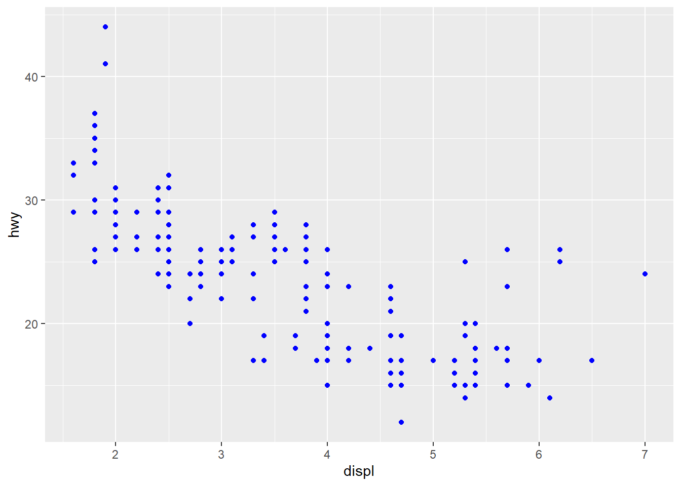

ggplot(data = mpg) +
    geom_point(mapping = aes(x = displ, y = hwy, color = class))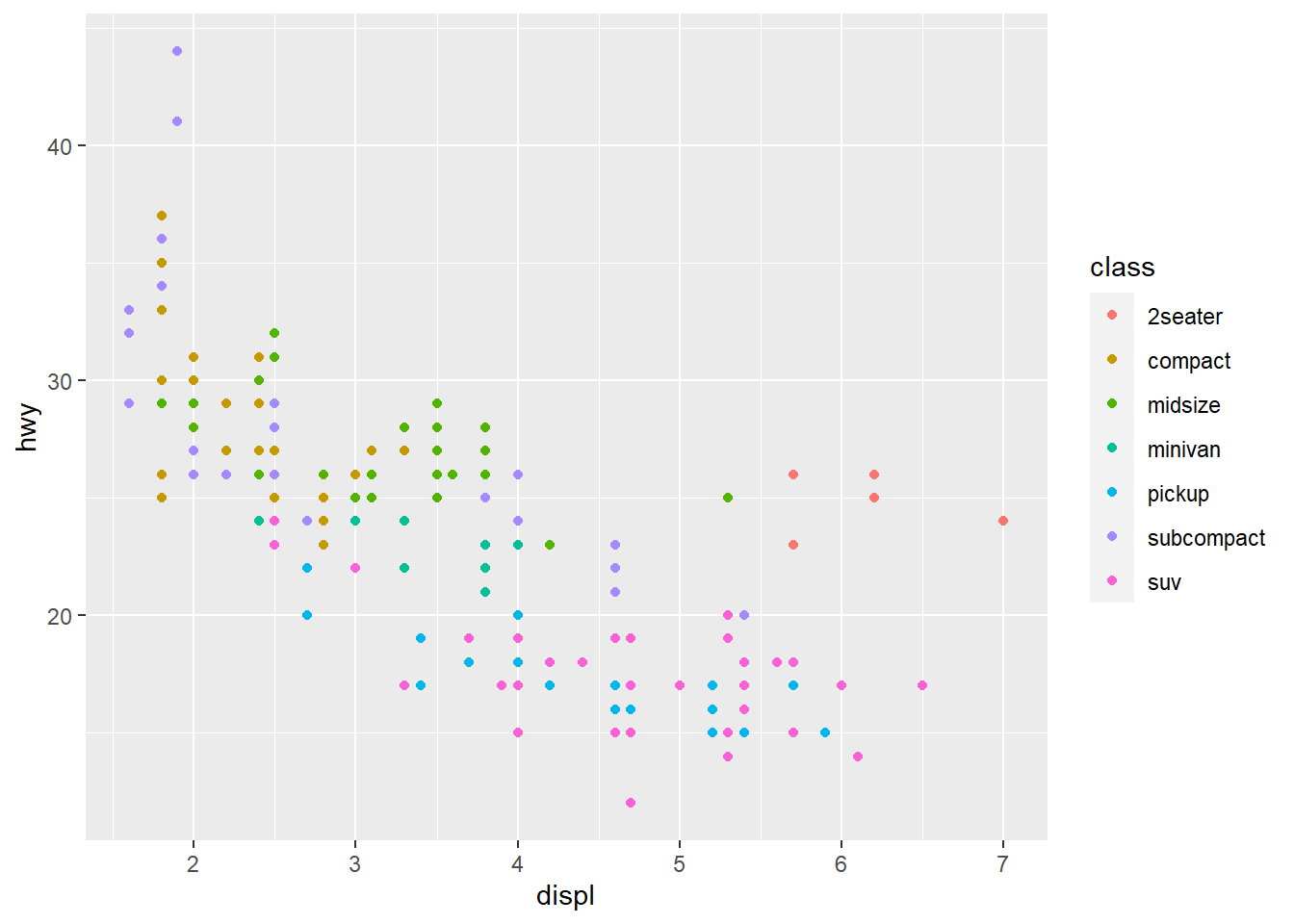

9.4.2 `facet`

For categorical data, you can split the plot into facets. This facet function will be attached as a layer followed by a + sign.

To facet your plot by a single variable, use facet_wrap(). The first argument should be a formula, which you create with ~ followed by a variable name.
To facet your plot by two variables, use facet_grid(). The first argument is a formula which contains two variable names separated by a ~.

Example 9.6

ggplot(data = mpg) +
    geom_point(mapping = aes(x = displ, y = hwy)) +
    facet_wrap(~ class, nrow = 2)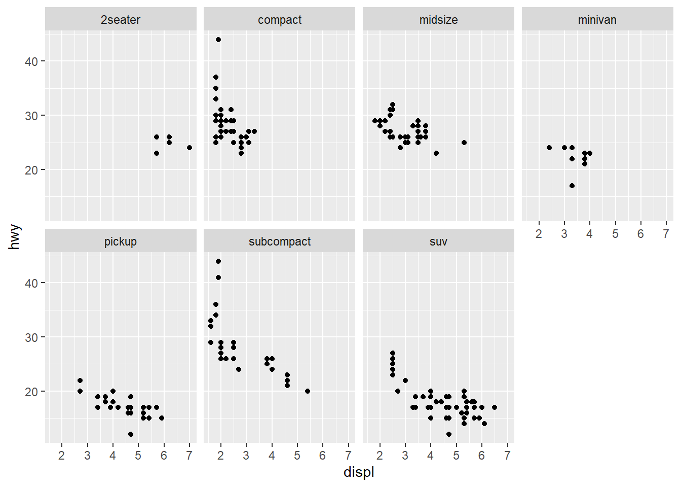

You may look at the variables to see the relations with the plot.

unique(mpg$class)
#> [1] "compact"    "midsize"    "suv"        "2seater"    "minivan"   
#> [6] "pickup"     "subcompact"

Example 9.7

ggplot(data = mpg) +
    geom_point(mapping = aes(x = displ, y = hwy)) +
    facet_grid(drv ~ cyl)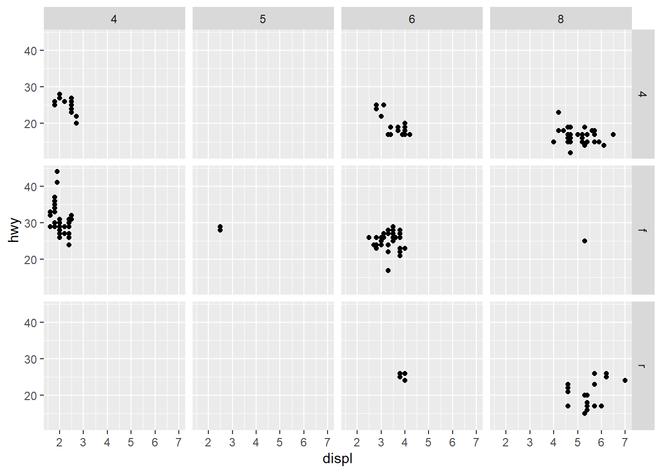

You may look at the variables to see the relations with the plot.

unique(mpg$drv)
#> [1] "f" "4" "r"
unique(mpg$cyl)
#> [1] 4 6 8 5

Tip

The ~ symbol is used to define a formula. The formula is a R object, which provide the pattern of a “formula”. Therefore drv~cyl means that drv is a function of cyl.

9.4.3 `geom` objects

A geom is the geometrical object that a plot uses to represent data. When drawing plots, you just need to attach those geometrical objects to a ggplot canvas with + symbol. Some of the geometrical objects can automatically do statistical transformations. The statistical transformations is short for stat, and the stat argument in those geom will show which statistical transformations are applied.

geom_point() draws scatter plot.
geom_smooth() draws smooth line approximation.
geom_bar() draws bar plot.
geom_histogram() draws histogram.

The arguments can be written in ggplot(). All the later geom will get those arguments from ggplot(). If the arguments are written again in geom object, it will override the ggplot() arguments.

Example 9.8

ggplot(data = mpg) +
    geom_point(mapping = aes(x = displ, y = hwy))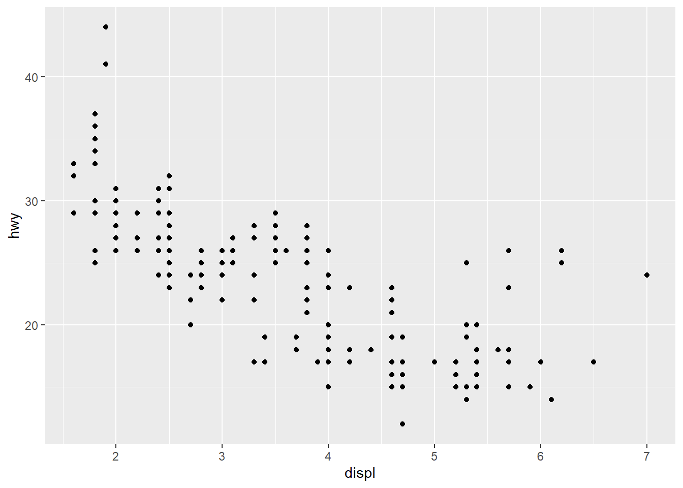


ggplot(data = mpg) +
    geom_smooth(mapping = aes(x = displ, y = hwy), formula = y ~ x, method = "loess")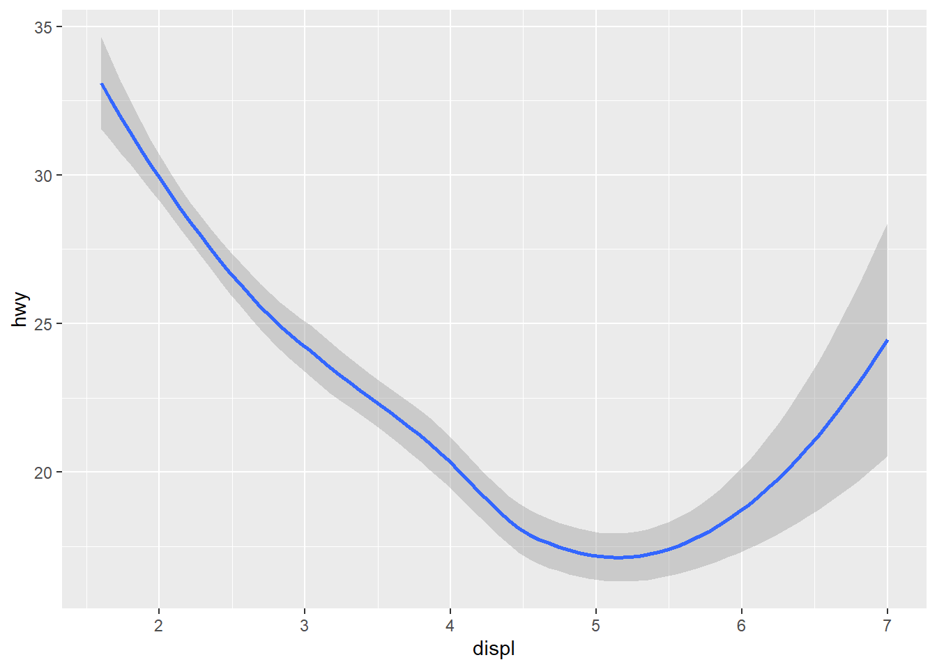


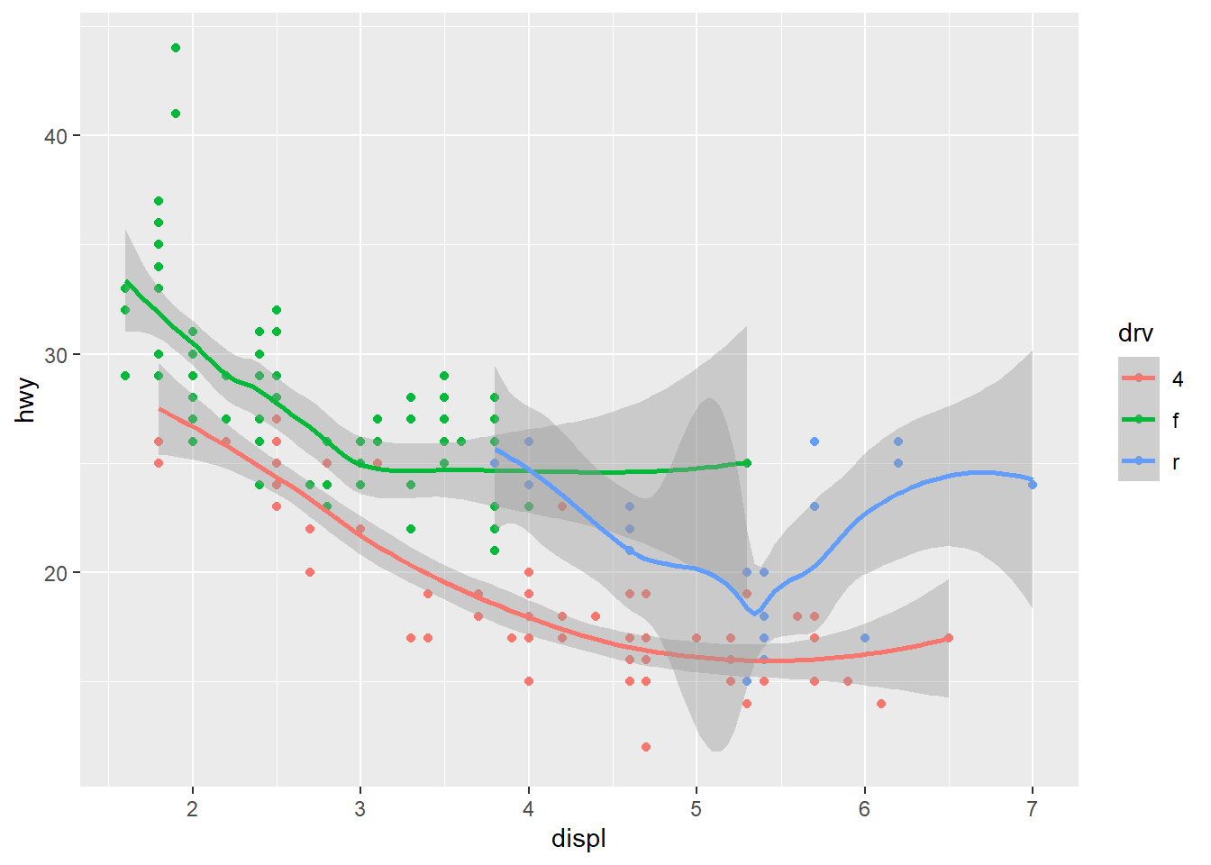
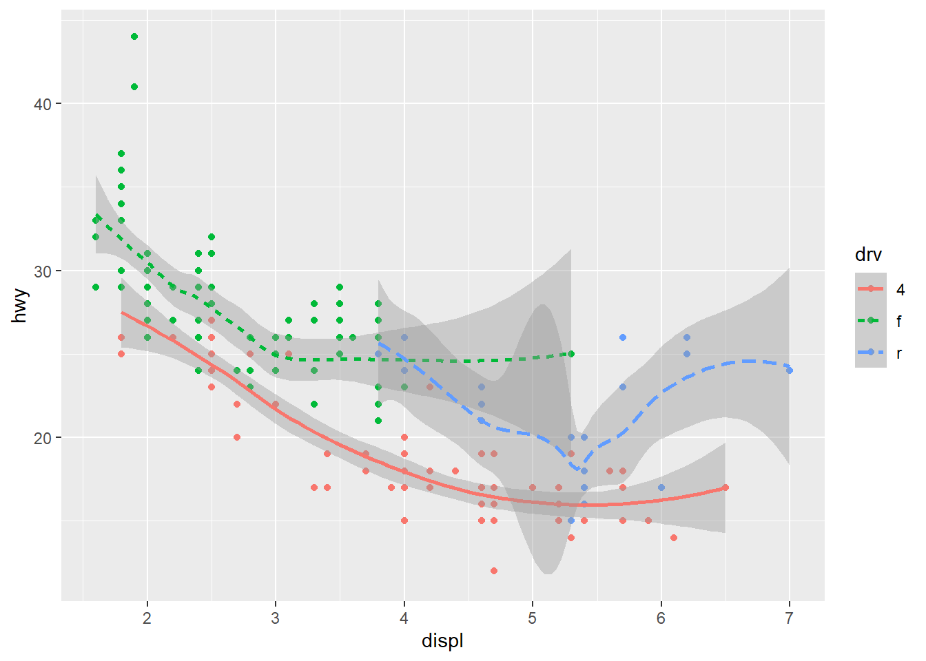
ggplot(data = mpg) +
    geom_smooth(mapping = aes(x = displ, y = hwy, linetype = drv), formula = y ~ x, method = "loess")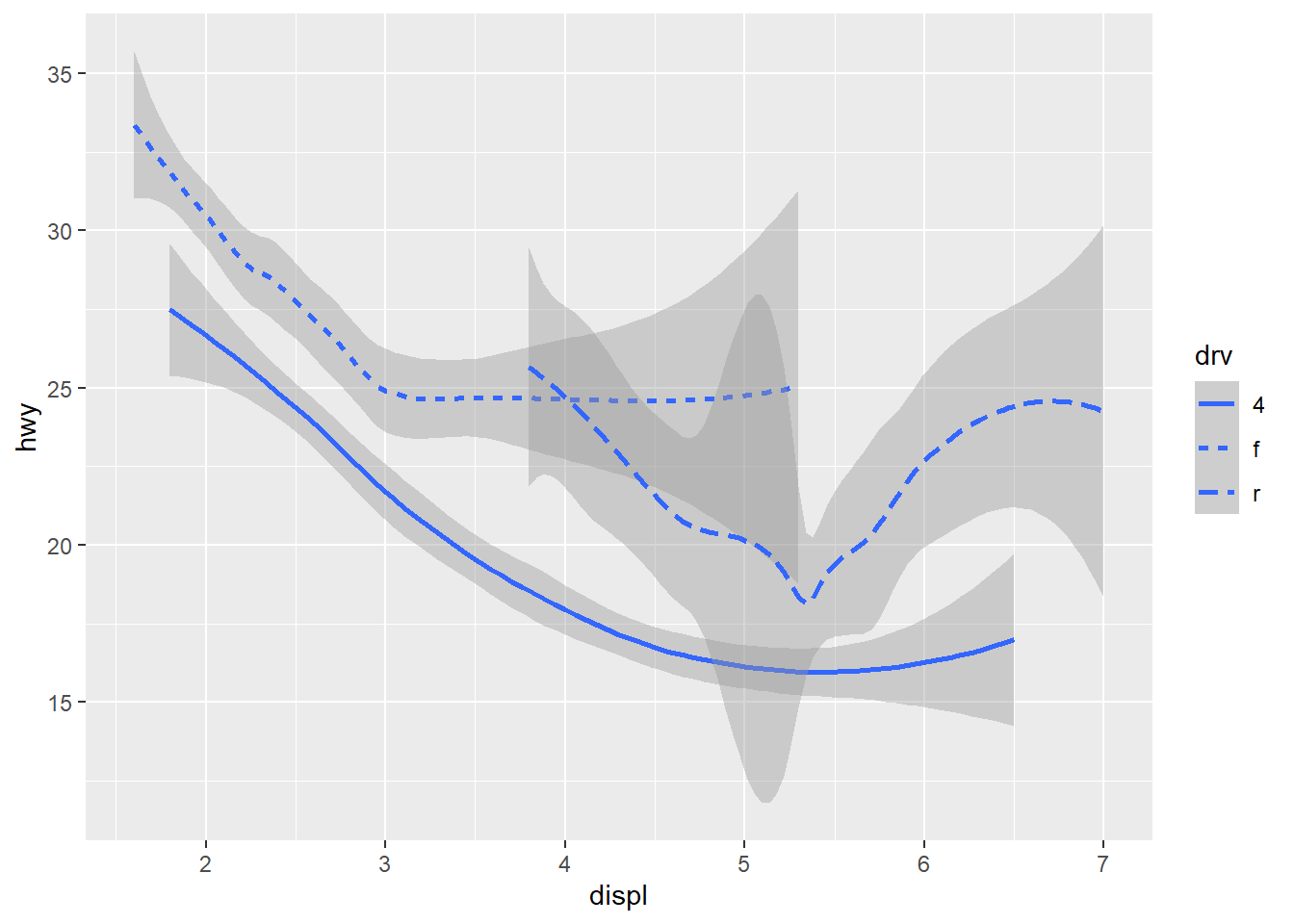


ggplot(data = mpg) +
    geom_point(mapping = aes(x = displ, y = hwy)) +
    geom_smooth(mapping = aes(x = displ, y = hwy), formula = y ~ x, method = "loess")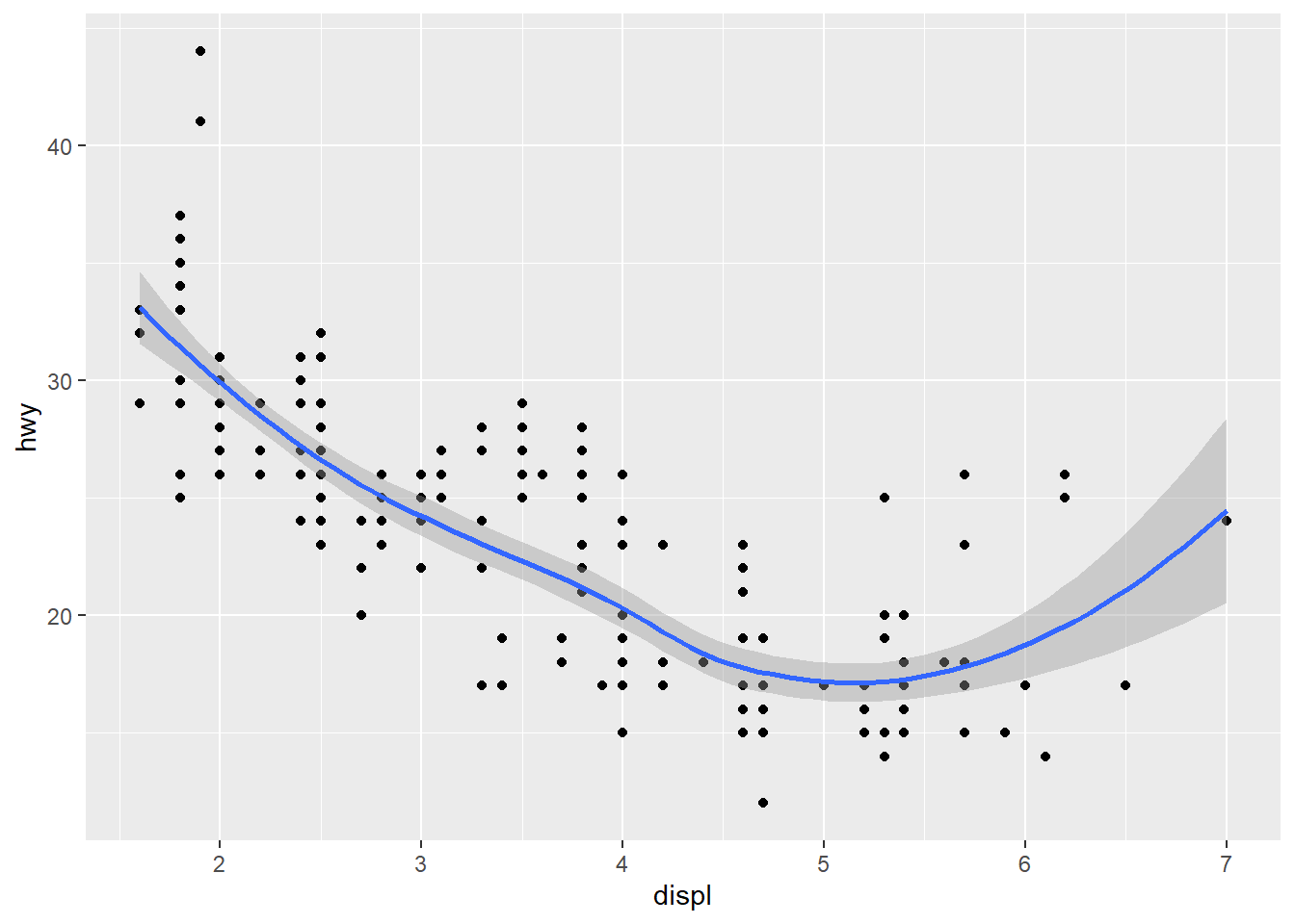


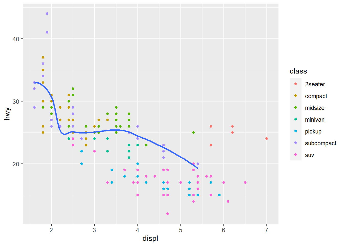
ggplot(data = mpg, mapping = aes(x = displ, y = hwy)) +
    geom_point(mapping = aes(color = class)) +
    geom_smooth(
        data = filter(mpg, class == "subcompact"),
        se = FALSE, 
        formula = y ~ x, method = "loess"
        )

9.5 Exercises

Exercise 9.1 How can you tell if an object is a tibble?

Exercise 9.2 Compare and contrast the following operations on a data.frame and equivalent tibble. What is different? Why might the default data frame behaviors cause you frustration?

df <- data.frame(abc = 1, xyz = "a")
df$x
df[, "xyz"]
df[, c("abc", "xyz")]

Exercise 9.3 If you have the name of a variable stored in an object, e.g., var <- "xyz", how can you extract the reference variable from a tibble? You may use the following codes to get a tibble.

tbl <- tibble(abc = 1, xyz = "a")

Exercise 9.4 Practice referring to nonsyntactic names in the following data.frame by:

Extracting the variable called 1.
Creating a new column called 3, which is 2 divided by 1.
Renaming the columns to one, two, and three:

annoying <- tibble(
`1` = 1:10,
`2` = `1` * 2 + rnorm(length(`1`))
)

Exercise 9.5 Both unite() and separate() have a remove argument. What does it do? Why would you set it to FALSE?

Exercise 9.6 Use flights dataset. Currently dep_time and sched_dep_time are convenient to look at, but hard to compute with because they’re not really continuous numbers. Convert them to a more convenient representation of number of minutes since midnight.

Exercise 9.7 Please make the following data tidy.

library(tidyverse)
df <- tibble(Day=1:5, `Plant_A_Height (cm)`=c(0.5, 0.7, 0.9, 1.3, 1.8), `Plant_B_Height (cm)`=c(0.7, 1, 1.5, 1.8, 2.2))

Exercise 9.8 Please use the flights dataset. Please find all flights that :

Had an arrival delay of two or more hours.
Flew to IAH or HOU.
Were operated by United, American or Delta.
Departed in summer (July, August, and September).
Arrived more than two hours late, but didn’t leave late.
Were delayed by at least an hour, but made up over 30 minutes in flight.
Departed between midnight and 6 a.m. (inclusive).

Exercise 9.9 Re-create the R code necessary to generate the following graphs. The dataset is mpg.

9.1 tibble

9.1.1 Create tibbles

9.1.2 Differences between tibble and data.frame.

9.1.2.1 Printing

9.1.2.2 Subsetting

9.1.3 %>% symbol

9.2 Tidy Data

9.2.1 Tidying datasets

9.2.1.1 pivot_longer()

9.2.1.2 pivot_wider()

9.2.1.3 separate()

9.2.1.4 unite()

9.3 dplyr

9.3.1 filter()

9.3.2 select()

9.3.3 mutate()

9.3.4 summarize() and group_by()

9.4 ggplot2

9.4.1 Aesthetic mappings

9.4.2 facet

9.4.3 geom objects

9.5 Exercises

9.1 `tibble`

9.1.3 `%>%` symbol

9.2.1.1 `pivot_longer()`

9.2.1.2 `pivot_wider()`

9.2.1.3 `separate()`

9.2.1.4 `unite()`

9.3 `dplyr`

9.3.1 `filter()`

9.3.2 `select()`

9.3.3 `mutate()`

9.3.4 `summarize()` and `group_by()`

9.4 `ggplot2`

9.4.2 `facet`

9.4.3 `geom` objects