4 Package: `pandas`

The basic data structure for pandas is pandas.DataFrame. You may treat it as a generalized version of tables.

To use pandas, we just import it. In most cases you would like to use the alias pd.

import pandas as pd

Since DataFrame is more like a table, the biggest questions here is not to do computations (which is still very important), but to retrieve, search, sort, merge, etc.. those data.

4.1 Basic `pandas`

4.1.1 `Series` and `DataFrame`

A Series is a 1-d array-like object which has index. The default index is starting from 0. You may change the index to be something assigned by you. Thus it can be treated as a generalization of a dict.

obj = pd.Series([3, 1, 2, 4])
obj

0    3
1    1
2    2
3    4
dtype: int64

obj2 = pd.Series([3, 1, 2, 4], index=['a', 'b', 'c', 'd'])
obj2

a    3
b    1
c    2
d    4
dtype: int64

data3 = {'a': 3, 'b': 1, 'c': 2, 'd': 4}
obj3 = pd.Series(data3)
obj3

a    3
b    1
c    2
d    4
dtype: int64

A DataFrame represents a rectangular table of data and contains an ordered collection of columns, each of which can be a different value type. The DataFrame has both a row and column index; it can be thought of as a dict of Series all sharing the same index. When displaying a DataFrame, we may use .head() to just display the first few rows for efficicy.

import pandas as pd

data = {'a': [1, 2, 3, 4, 5, 6, 7],
        'b': [1.1, 2.1, 3.1, 4.1, 5.1, 6.1, 7.1],
        'c': ['a', 'b', 'c', 'd', 'e', 'f', 'g']}
df = pd.DataFrame(data)
df.head()

	a	b	c
0	1	1.1	a
1	2	2.1	b
2	3	3.1	c
3	4	4.1	d
4	5	5.1	e

4.1.2 Decorations

A Series or a DataFrame might have named row indexes and column names. I collect some tools for you to play with them and list them below.

Setting when creating

We may use the setting columns= or index= to change the column names and the index names. See the following example.

import numpy as np
import pandas as pd
data = pd.DataFrame(np.arange(16).reshape((4, 4)),
                    index=['Ohio', 'Colorado', 'Utah', 'New York'],
                    columns=['one', 'two', 'three', 'four'])
data

	one	two	three	four
Ohio	0	1	2	3
Colorado	4	5	6	7
Utah	8	9	10	11
New York	12	13	14	15

.rename()

We may use the .rename() method. Note that by default the return value of this method is a copy and it won’t affect the original DataFrame. The arguments can be in many different formats. Please see the official document for more details.

If you want to directly make the change, please use the argument inplace=True.

The following example shows the standard way to rename.

df = pd.DataFrame(np.arange(16).reshape((4, 4)))
df.rename(columns={0: 'zero'}, index={2: 'two'})

	zero	1	2	3
0	0	1	2	3
1	4	5	6	7
two	8	9	10	11
3	12	13	14	15

However the orginal df is not affected.

df

	0	1	2	3
0	0	1	2	3
1	4	5	6	7
2	8	9	10	11
3	12	13	14	15

If you would like to change the original df, you may either set df = df.rename(columns={0: 'zero'}, index={2: 'two'}), or

df.rename(columns={0: 'zero'}, index={2: 'two'}, inplace=True)
df

	zero	1	2	3
0	0	1	2	3
1	4	5	6	7
two	8	9	10	11
3	12	13	14	15

Set a column to be the index by .set_index()

The title is all. A few remarks:

You may set multiple columns to be the index. In this case, what you get is a multi-index system (which is also called Hierarchical indexing). We will talk about this later in Section 4.4.2.
The argument drop is used to control whether the column is deleted after you set it to be the index. The default setting is True.
The argument append is used to control whether the column you choose is appended to the exsiting index to form a multi-index system. The default is False.
The argument inplace is used to control whether you want to make the change inplace. The default is False.

Reset the index by .reset_index()

The title is all. A few remarks:

The new index is integers starting from 0.
drop is an argument to control whether the original index is dropped or added back to the DataFrame as a column. The default is False, which means that by default the original index will be added back to the DataFrame.

4.1.3 Look at the `DataFrame`

The following methods can be used to look at the DataFrame. Their syntax is very simple. Please try them by yourselves.

.head(): show the first few rows.
.tail(): show the last few rows.
.describe(): show the basic statistics of each columns.

These are methods for Series which might be helpful to understand the data.

.unique()
.value_counts()

An example

import pandas as pd

df = pd.DataFrame({'a': [1, 2, 3, 1, 2, 2, 1, 1, 1],
                   'b': [3, 1, 1, 2, 4, 5, 2, 1, 3]})
df.head(3)

	a	b
0	1	3
1	2	1
2	3	1

df.tail()

	a	b
4	2	4
5	2	5
6	1	2
7	1	1
8	1	3

df.describe()

	a	b
count	9.000000	9.000000
mean	1.555556	2.444444
std	0.726483	1.424001
min	1.000000	1.000000
25%	1.000000	1.000000
50%	1.000000	2.000000
75%	2.000000	3.000000
max	3.000000	5.000000

df['a'].unique()

array([1, 2, 3], dtype=int64)

df['b'].value_counts()

1    3
3    2
2    2
4    1
5    1
Name: b, dtype: int64

4.2 Indexing

The act of selecting rows or columns to access from a dataframe or series is called indexing. There are many different ways to index in pandas. We will only cover the most popular ones.

Caution

There is the same copy and view issue with pandas as in numpy. However it is more complicated and more inconsistent. Please check the official documents for more details and do more experiments before implementing the codes. Usually if your code is ambiguous, you might see the infamous SettingWithCopyWarning warning.

df = pd.DataFrame({'a': [1, 2, 3], 'b': [4, 5, 6]})
df[df['a']==3]['b'] = 3

C:\Users\Xinli\AppData\Local\Temp\ipykernel_10540\4018622545.py:2: SettingWithCopyWarning: 
A value is trying to be set on a copy of a slice from a DataFrame.
Try using .loc[row_indexer,col_indexer] = value instead

See the caveats in the documentation: https://pandas.pydata.org/pandas-docs/stable/user_guide/indexing.html#returning-a-view-versus-a-copy
  df[df['a']==3]['b'] = 3

Note that pandas is testing a copy-on-write feature to fix the issue. The feature can be simlified as “any DataFrame or Series derived from another in any way always behaves as a copy”. Please keep an eye on the updates about when the feature will be fully implemented in pandas.

4.2.1 `[]`

Series[]

Input value type	Return Value Type
`Series[label]`	scalar value
`Series[list of labels]`	`Series` corresponding to labels
`Series[slice]`	`Series` corresponding to the slice
`Series[boolean vector]`	`Series` corresponding to the boolean vector

For Series, values are accessed by labels, not positions. Since Series are usually considered as a column, you may think these labels as row indexes.
When using slice, things becomes more complicated. There are two ways of using slice. You may either slice by positions, or slice by labels. The main differences between them is that:

slice by positions Series[i:j] doesn’t contain the last index Series[j];
slice by labels Sereies[I:J] contains the last label Series[J].

Sometimes the labels of a series are integers, but different than the position indexes. In pandas 1.5.1, slice by positions takes priority. However the whole scenario is very confusing, and this will be changed in future versions. In this cases it is recommanded to use .loc and .iloc.
When indexing using boolean vector, the vector should be of the same length as the Series. In other words, it works as the boolean bector shows which row is selected.

See some examples below.

Example 4.1

import pandas as pd

example = pd.Series({'a': 1.1, 'b': 2.2, 'c': 3.3, 'd': 4.4})
example

a    1.1
b    2.2
c    3.3
d    4.4
dtype: float64

example['b']

2.2

example[['b', 'a']]

b    2.2
a    1.1
dtype: float64

example[0:2]

a    1.1
b    2.2
dtype: float64

example['a':'c']

a    1.1
b    2.2
c    3.3
dtype: float64

example[[True, False, True, False]]

a    1.1
c    3.3
dtype: float64

DataFrame[]

Input value type	Return Value Type
`DataFrame[colname]`	The column corresponding to colname as a `Series`
`DataFrame[list-of-colnames]`	The columns of `DataFrame` corresponding to colnames
`DataFrame[slice]`	The rows of `DataFrame` corresponding to the slice
`DataFrame[boolean list]`	`DataFrame` corresponding to the boolean list

Slice for DataFrame behaves exactly like slice for Series, that it is selecting rows, and it works for both labels and positions. Similarly, slicing by positions are not recommended and might be deprecated in the future.
On the other hand side, selecting rows are usually related to querying. Therefore it is better not to focus on slicing.
Inside [], one column name and a list of columna names will result totally different objects: one is a Series and the other is a DataFrame.
In prior versions, using [list-of-colnames] would work as long as at least 1 of the keys was found (otherwise it would raise a KeyError). This behavior was changed and will now raise a KeyError if at least one label is missing. The recommended alternative is to use .reindex().
When indexing using boolean vector, the vector should be of the same length as the number of rows of the DataFrame. In other words, it works as the boolean bector shows which row is selected.
Using [] for DataFrame cannot give you a single value, since what are inside [] is always treated as a row index or a column index. If you want to get access to the value of a single cell by both row index and column index, use other method like .loc[].
If the column name is eligible for attributes, you may also use df.a to represent df['a'] for simplicity.

Example 4.2

import pandas as pd

example = pd.DataFrame({'a': [1.1, 2.2], 'b': [2.2, 3.3], 'c': [3.3, 4.4]})
example

	a	b	c
0	1.1	2.2	3.3
1	2.2	3.3	4.4

example['a']

0    1.1
1    2.2
Name: a, dtype: float64

example.a

0    1.1
1    2.2
Name: a, dtype: float64

example[['a']]

	a
0	1.1
1	2.2

example[0:1]

	a	b	c
0	1.1	2.2	3.3

example[[False, True]]

	a	b	c
1	2.2	3.3	4.4

4.2.2 `.loc[]` and `.iloc[]`

[] contains several different types of ways to access data. .loc[] and .iloc[] are more specific.

.loc[] is to use labels to access data.
.iloc[] is to use positions to access data.

Notes for .loc[] and .iloc[]

When there is only one index is specified, it is refered to rows.
When using both indexes, the first is row index and the second is column index.
When selecting all rows/columns, you may put : in the corresponding place.
df.loc[1, 'a'] refers to the cell in the DataFrame df whose row index is 1 and column index is a. df[1, 'a'] refers to the column in the DataFrame df whose column name is (1, 'a').
Many other small details are very similar to []. For example, pay attention to the differences between df.loc[:, 'a'] and df.loc[:, ['a']].

Example 4.3

import pandas as pd
example = pd.DataFrame({'a': [1.1, 2.2], 'b': [2.2, 3.3], 'c': [3.3, 4.4]})
example

	a	b	c
0	1.1	2.2	3.3
1	2.2	3.3	4.4

example.loc[1]

a    2.2
b    3.3
c    4.4
Name: 1, dtype: float64

example.loc[:, 'a']

0    1.1
1    2.2
Name: a, dtype: float64

example.loc[1, 'a']

2.2

example.iloc[0:1, 0:2]

	a	b
0	1.1	2.2

example.iloc[1, 0:2]

a    2.2
b    3.3
Name: 1, dtype: float64

example.iloc[[1], 0:2]

	a	b
1	2.2	3.3

4.2.3 Boolean indexing

Let df be a DataFrame. Assume that boo is boolean vector of the dimension same to the number of rows of df, then we can use df[boo] to filter data: all rows with True will be selected. The syntax is similar to the boolean indexing in numpy.

The basic usage of boolean indexing

import pandas as pd
import numpy as np
df = pd.DataFrame(np.random.randn(8, 4),
                  index=pd.date_range('1/1/2023', periods=8),
                  columns=['A', 'B', 'C', 'D'])
df

	A	B	C	D
2023-01-01	0.237607	1.323886	-0.658127	-0.975299
2023-01-02	-0.764331	0.833129	-2.136817	-0.494983
2023-01-03	-0.857309	-0.025589	0.802247	-0.437641
2023-01-04	0.833024	-0.345832	-0.224655	-1.669289
2023-01-05	-0.610940	0.804115	-0.147965	-1.162376
2023-01-06	1.149887	-1.471409	-1.546448	0.805580
2023-01-07	1.150973	-2.067331	-1.544236	-0.131534
2023-01-08	0.208735	-0.331659	-1.371364	0.762330

df[df['A']>0]

	A	B	C	D
2023-01-01	0.237607	1.323886	-0.658127	-0.975299
2023-01-04	0.833024	-0.345832	-0.224655	-1.669289
2023-01-06	1.149887	-1.471409	-1.546448	0.805580
2023-01-07	1.150973	-2.067331	-1.544236	-0.131534
2023-01-08	0.208735	-0.331659	-1.371364	0.762330

To get the boolean vector, we may directly compute logic expression using columns of df. The previous example is of this kind.

You may write complicated expressions. The operators are:

| for or
& for and
~ for not

Note that parentheses must be used to ensure a correct result. Please see the following example.

df[(df['A'] > 1) & (df['B'] < 3)]

	A	B	C	D
2023-01-06	1.149887	-1.471409	-1.546448	0.805580
2023-01-07	1.150973	-2.067331	-1.544236	-0.131534

There are many methods and functions that can create boolean vectors. We will introduce them when we need them.

4.2.4 `.query()`

DataFrame has a .query() method that allows filtering using an expression instead of a boolean vector. This method uses a different approach from the point of programming language. From the point of users, you are free to choose between .query() and boolean indexing to filter data.

Here are examples of .query().

df = pd.DataFrame({'A': [1,2,3], 'B': [3,2,1], 'C': [5,4,3]})
df

	A	B	C
0	1	3	5
1	2	2	4
2	3	1	3

df.query('A<B and B<C')

	A	B	C
0	1	3	5

It can be simplified as follows:

df.query('A<B<C')

	A	B	C
0	1	3	5

This is the same as the following code.

df[(df['A']<df['B']) & (df['B']<df['C'])]

	A	B	C
0	1	3	5

Note that .query() does not require the usage of parentheses. It also use English like or/and/not for |/&/~.

df.query('A in C')

	A	B	C
2	3	1	3

df.query('A not in C')

	A	B	C
0	1	3	5
1	2	2	4

df.query('A not in C and A<B')

	A	B	C
0	1	3	5

df.query('[1,2] in B')

	A	B	C
1	2	2	4
2	3	1	3

4.2.5 Reindex

.reindex() is a data alignment method in pandas. To reindex means to conform the data to match a given set of labels along a particular axis. This accomplishes several things:

Reordering the existing data to match a new set of labels
Inserting missing value (NaN) markers in label locations where no data for that label existed

Here is a simple example:

import pandas as pd
data = pd.DataFrame(np.arange(16).reshape((4, 4)),
                    index=['Ohio', 'Colorado', 'Utah', 'New York'],
                    columns=['one', 'two', 'three', 'four'])
data

	one	two	three	four
Ohio	0	1	2	3
Colorado	4	5	6	7
Utah	8	9	10	11
New York	12	13	14	15

data.reindex(index = ['Colorado', 'Arkansas', 'New York'],
             columns = ['three', 'five', 'one'])

	three	five	one
Colorado	6.0	NaN	4.0
Arkansas	NaN	NaN	NaN
New York	14.0	NaN	12.0

From the first glance, .reindex() behave the same as other indexing methods. Here are a few differences:

The purpose of indexing methods is to select/filter data, while the purpose of reindex is to make the data in a very specific form.
When dealing with non-existent indexes/columns, most other indexing methods will return error or warning, while .reindex() can handle it automatically.
The default setting of .reindex() is to return a copy. This setting can be changed by the argument copy=False.

For more details please see the official guide.

4.2.6 Updating data

Assign values to a column of a DataFrame will update that column. If the column doesn’t exist, new column will be created. This is called enlargement.
When assign values with non-existent row index, that part of the data will be discarded.
When using .loc, a DataFrame can be enlarged on either axis.
Any time if there are no values with a specific column and row, it will show as NaN.

Example 4.4

import pandas as pd

data = {'a': [1, 2, 3, 4],
        'b': [1.1, 2.1, 3.1, 4.1],
        'c': ['a', 'b', 'c', 'd']}
df = pd.DataFrame(data)

newcol = {1: 'good', 3: 'better', 5: 'best'}
df['d'] = pd.Series(newcol)
df

	a	b	c	d
0	1	1.1	a	NaN
1	2	2.1	b	good
2	3	3.1	c	NaN
3	4	4.1	d	better

4.3 Data cleaning

4.3.1 Handling Missing Data

np.nan, pd.NA
pd.isnull(), np.isnan()
.dropna(), .fillna()

.dropna() example

import pandas as pd
import numpy as np

data = pd.DataFrame([[1., 6.5, 3.], [1., np.nan, np.nan], 
                     [np.nan, np.nan, np.nan], [np.nan, 6.5, 3.]])
data

	0	1	2
0	1.0	6.5	3.0
1	1.0	NaN	NaN
2	NaN	NaN	NaN
3	NaN	6.5	3.0

data.dropna()

	0	1	2
0	1.0	6.5	3.0

data.dropna(how='all')

	0	1	2
0	1.0	6.5	3.0
1	1.0	NaN	NaN
3	NaN	6.5	3.0

data[4] = np.nan
data

	0	1	2	4
0	1.0	6.5	3.0	NaN
1	1.0	NaN	NaN	NaN
2	NaN	NaN	NaN	NaN
3	NaN	6.5	3.0	NaN

data.dropna(axis=1, how='all')

	0	1	2
0	1.0	6.5	3.0
1	1.0	NaN	NaN
2	NaN	NaN	NaN
3	NaN	6.5	3.0

data.dropna(thresh=2)

	0	1	2	4
0	1.0	6.5	3.0	NaN
3	NaN	6.5	3.0	NaN

.fillna() example

data.fillna(0)

	0	1	2
0	1.0	6.5	3.0
1	1.0	0.0	0.0
2	0.0	0.0	0.0
3	0.0	6.5	3.0

data.fillna({1: 0.5, 2: -0.1})

	0	1	2	4
0	1.0	6.5	3.0	NaN
1	1.0	0.5	-0.1	NaN
2	NaN	0.5	-0.1	NaN
3	NaN	6.5	3.0	NaN

Arithmetic and Data Alignment

Elements of the same index and columns will be computed. By default, if any entry is nan, the answer will be nan. You may use fill_value argument to fill the empty slots. Please see the following example.

import pandas as pd
import numpy as np
df1 = pd.DataFrame(np.arange(12.).reshape((3, 4)), columns=list('abcd'))
df2 = pd.DataFrame(np.arange(20.).reshape((4, 5)), columns=list('abcde'))
df2.loc[1, 'b'] = np.nan

df1.add(df2, fill_value=0)

	a	b	c	d	e
0	0.0	2.0	4.0	6.0	4.0
1	9.0	5.0	13.0	15.0	9.0
2	18.0	20.0	22.0	24.0	14.0
3	15.0	16.0	17.0	18.0	19.0

Relatedly, when reindexing a Series or DataFrame, you can also specify a fill_value.

4.3.2 Handling duplicates

.drop_duplicates() example

import numpy as np
import pandas as pd

data = pd.DataFrame({'k1': ['one', 'two'] * 3 + ['two'], 
                     'k2': [1, 1, 2, 3, 3, 4, 4]})
data.drop_duplicates(['k1'], keep='last')

	k1	k2
4	one	3
6	two	4

4.3.3 Drop data

You may use .drop() to drop columns or rows.

If you directly apply .drop() to an index, that index is considered as a row index.
To drop a column, you need to specify the argument columns=.
There is still the inplace= issue.

4.3.4 String Manipulation

When the column Series is of type str, all methods in pd.Series.str will be applied to each entry of the Series.

Some basic examples

import pandas as pd
import numpy as np
s = pd.Series(["A ", " B ", "C", "Aaba", " Baca ", np.nan, "CABA", "dog", "cat"])
s

0        A 
1        B 
2         C
3      Aaba
4     Baca 
5       NaN
6      CABA
7       dog
8       cat
dtype: object

s.str.lower()

0        a 
1        b 
2         c
3      aaba
4     baca 
5       NaN
6      caba
7       dog
8       cat
dtype: object

s.str.split('a')

0          [A ]
1         [ B ]
2           [C]
3      [A, b, ]
4    [ B, c,  ]
5           NaN
6        [CABA]
7         [dog]
8        [c, t]
dtype: object

s.str.len()

0    2.0
1    3.0
2    1.0
3    4.0
4    6.0
5    NaN
6    4.0
7    3.0
8    3.0
dtype: float64

s.str.strip()

0       A
1       B
2       C
3    Aaba
4    Baca
5     NaN
6    CABA
7     dog
8     cat
dtype: object

s.str.replace("A", '1')

0        1 
1        B 
2         C
3      1aba
4     Baca 
5       NaN
6      C1B1
7       dog
8       cat
dtype: object

Example 4.5 We could also use .str to play with column names and row indexes.

import pandas as pd
import numpy as np
df = pd.DataFrame(np.random.randn(3, 2),
                  columns=[" Column A ", " Column B "], index=range(3))

df.columns = df.columns.str.strip().str.lower().str.replace(' ', '_')
df

	column_a	column_b
0	0.465369	1.539442
1	2.196586	-1.541876
2	0.371981	0.309551

String methods are usually used with regular expressions. For more details please see Appendix F.

4.4 Data Wrangling

4.4.1 Tidy data

The same underlying data can be represented in multiple ways. To better study the data, it is better to make these data tidy.

Definition 4.1 A dataset is tidy if

Each variable have its own column.
Each observation have its own row.
Each value have its oven cell.

Typical examples of tidydata

These DataFrame are provided by tidyr. We will talk about them again when we get to R. These tables can be downloaded by clicking the names.

table1

import pandas as pd
table1 = pd.read_csv('assests/datasets/table1.csv', index_col='Unnamed: 0')
table1

	country	year	cases	population
1	Afghanistan	1999	745	19987071
2	Afghanistan	2000	2666	20595360
3	Brazil	1999	37737	172006362
4	Brazil	2000	80488	174504898
5	China	1999	212258	1272915272
6	China	2000	213766	1280428583

table2

import pandas as pd
table2 = pd.read_csv('assests/datasets/table2.csv', index_col='Unnamed: 0')
table2

	country	year	type	count
1	Afghanistan	1999	cases	745
2	Afghanistan	1999	population	19987071
3	Afghanistan	2000	cases	2666
4	Afghanistan	2000	population	20595360
5	Brazil	1999	cases	37737
6	Brazil	1999	population	172006362
7	Brazil	2000	cases	80488
8	Brazil	2000	population	174504898
9	China	1999	cases	212258
10	China	1999	population	1272915272
11	China	2000	cases	213766
12	China	2000	population	1280428583

table3

import pandas as pd
table3 = pd.read_csv('assests/datasets/table3.csv', index_col='Unnamed: 0')
table3

	country	year	rate
1	Afghanistan	1999	745/19987071
2	Afghanistan	2000	2666/20595360
3	Brazil	1999	37737/172006362
4	Brazil	2000	80488/174504898
5	China	1999	212258/1272915272
6	China	2000	213766/1280428583

Spread across two DataFrames: table4a and table4b:

import pandas as pd
table4a = pd.read_csv('assests/datasets/table4a.csv', index_col='Unnamed: 0')
table4b = pd.read_csv('assests/datasets/table4b.csv', index_col='Unnamed: 0')
table4a

	country	1999	2000
1	Afghanistan	745	2666
2	Brazil	37737	80488
3	China	212258	213766

table4b

	country	1999	2000
1	Afghanistan	19987071	20595360
2	Brazil	172006362	174504898
3	China	1272915272	1280428583

Among all these DataFrames, only table1 is tidy.

These three conditions are interrelated because it is impossible to only satisfy two of the three. In pratical, we need to follow the instructions:

Put each dataset in a DataFrame.
Put each variable in a column.
Every row is about one obeservation.

Tidy data is a consistent way to organize your data. The main advantages are:

It is one consistent way of storing data. In other words, this is a consistent data structure that can be used in many cases.
To placing variables in columns enables Python to do vectorized operations.

Most datasets are untidy, since tidy data is usually not intuitive for collecting. Therefore raw data which are collected by some naive ideas are usually not tidy.

Untidy data are usually:

One variable might be spread across multiple columns.
One observation might be scattered across multiple rows.

.melt() method

A common problem is that the column names are not names of variables, but values of a variable. For example, table4a above has columns 1999 and 2000. These two names are actually the values of a variable year. In addition, each row represents two observations, not one.

	country	1999	2000
1	Afghanistan	745	2666
2	Brazil	37737	80488
3	China	212258	213766

To tidy this type of dataset, we need to gather those columns into a new pair of variables. We need three parameters:

The set of columns that represent values. In this case, those are 1999 and 2000.
The name of the variable. In this case, it is year. -The name of the variable whose values are spread over the cells. In this case, it is the number of cases.

Then we apply .melt().

table4a.melt(id_vars=['country'],
             value_vars=['1999', '2000'],
             var_name='year',
             value_name='cases')

	country	year	cases
0	Afghanistan	1999	745
1	Brazil	1999	37737
2	China	1999	212258
3	Afghanistan	2000	2666
4	Brazil	2000	80488
5	China	2000	213766

We can do the similar thing to table4b.

table4b.melt(id_vars=['country'],
             value_vars=['1999', '2000'],
             var_name='year',
             value_name='population')

	country	year	population
0	Afghanistan	1999	19987071
1	Brazil	1999	172006362
2	China	1999	1272915272
3	Afghanistan	2000	20595360
4	Brazil	2000	174504898
5	China	2000	1280428583

Tip

In Python there are multiple different ways to change a wide DataFrame to be longer like .melt(). Among all of them, .melt() is the most common one.

.pivot() method

Another issuse is that an observation is scattered across multiple rows. Take table2 as an example.

An observation is a country in a year, but each observation is spread across two rows.

table2

	country	year	type	count
1	Afghanistan	1999	cases	745
2	Afghanistan	1999	population	19987071
3	Afghanistan	2000	cases	2666
4	Afghanistan	2000	population	20595360
5	Brazil	1999	cases	37737
6	Brazil	1999	population	172006362
7	Brazil	2000	cases	80488
8	Brazil	2000	population	174504898
9	China	1999	cases	212258
10	China	1999	population	1272915272
11	China	2000	cases	213766
12	China	2000	population	1280428583

We could apply .pivot() to make it tidy. Here we need two arguments.

The column that contains variable names. Here, it’s type.
The column that contains values forms multiple variables. Here, it’s count.

table2.pivot(index=['country', 'year'], columns='type', values='count')

	type	cases	population
country	year
Afghanistan	1999	745	19987071
Afghanistan	2000	2666	20595360
Brazil	1999	37737	172006362
Brazil	2000	80488	174504898
China	1999	212258	1272915272
China	2000	213766	1280428583

Split and combine columns

If we would like to split one columns into multiple columns since there are more than one values in a cell, we could use Series string method to split it.

table3['newrate'] = table3['rate'].str.split('/')
table3

	country	year	rate	newrate
1	Afghanistan	1999	745/19987071	[745, 19987071]
2	Afghanistan	2000	2666/20595360	[2666, 20595360]
3	Brazil	1999	37737/172006362	[37737, 172006362]
4	Brazil	2000	80488/174504898	[80488, 174504898]
5	China	1999	212258/1272915272	[212258, 1272915272]
6	China	2000	213766/1280428583	[213766, 1280428583]

If we prepare two columns from the beginning, we could directly get two columns. Note that the argument expand=True means that we want to get a DataFrame by expanding dimensionality. More details can be found here.

table3[['cases', 'population']] = table3['rate'].str.split('/', expand=True)
table3.drop(columns=['rate', 'newrate'], inplace=True)
table3

	country	year	cases	population
1	Afghanistan	1999	745	19987071
2	Afghanistan	2000	2666	20595360
3	Brazil	1999	37737	172006362
4	Brazil	2000	80488	174504898
5	China	1999	212258	1272915272
6	China	2000	213766	1280428583

Similarly we could also combine columns just as they are strings.

table3['another_rate'] = table3['cases']+'/'+table3['population']
table3

	country	year	cases	population	another_rate
1	Afghanistan	1999	745	19987071	745/19987071
2	Afghanistan	2000	2666	20595360	2666/20595360
3	Brazil	1999	37737	172006362	37737/172006362
4	Brazil	2000	80488	174504898	80488/174504898
5	China	1999	212258	1272915272	212258/1272915272
6	China	2000	213766	1280428583	213766/1280428583

4.4.2 Hierarchical indexing

Pandas support a more complex indexing system, that the index may have multiple levels. See the following example.

An example

import pandas as pd
import numpy as np

data = pd.Series(np.random.randn(9),
                 index = [['a', 'a', 'a', 'b', 'b', 'c', 'c', 'd', 'd'],
                          [1, 2, 3, 1, 2, 3, 1, 2, 3]])
data

a  1   -0.729463
   2   -0.550397
   3    1.271335
b  1   -0.139672
   2   -0.083897
c  3    0.699671
   1    0.184548
d  2   -0.414853
   3    0.931543
dtype: float64

You may look at the Series using different levels of indexes.

data['a']

1   -0.729463
2   -0.550397
3    1.271335
dtype: float64

data.loc[:, 2]

a   -0.550397
b   -0.083897
d   -0.414853
dtype: float64

You may use groupby to group by levels and do calculations related to levels. More .groupby() will be discussed in the next section.

data.groupby(level=1).sum()

1   -0.684587
2   -1.049147
3    2.902549
dtype: float64

From the example above, you may notice that the 2-level hierarchical indexing for a Series works very similar to a DataFrame. In fact, you may translate it back and forth between a 2-level indexing Series and a DataFrame.

df = data.unstack()
df

	1	2	3
a	-0.729463	-0.550397	1.271335
b	-0.139672	-0.083897	NaN
c	0.184548	NaN	0.699671
d	NaN	-0.414853	0.931543

df.stack()

a  1   -0.729463
   2   -0.550397
   3    1.271335
b  1   -0.139672
   2   -0.083897
c  1    0.184548
   3    0.699671
d  2   -0.414853
   3    0.931543
dtype: float64

For DataFrame the index for both axes can be multiindex. The usual indexing way can be used if you want to start from the first level of the index. The more specific method to extract data is .xs.

An example

import pandas as pd

df1 = pd.DataFrame(
    {
        "A": ["A0", "A1", "A2", "A3"],
        "B": ["B0", "B1", "B2", "B3"],
        "C": ["C0", "C1", "C2", "C3"],
        "D": ["D0", "D1", "D2", "D3"],
    },
    index=[0, 1, 2, 3],
)

df2 = pd.DataFrame(
    {
        "A": ["A4", "A5", "A6", "A7"],
        "B": ["B4", "B5", "B6", "B7"],
        "C": ["C4", "C5", "C6", "C7"],
        "D": ["D4", "D5", "D6", "D7"],
    },
    index=[4, 5, 6, 7],
)

df = pd.concat([df1, df2], keys=['x', 'y'])

df

		A	B	C	D
x	0	A0	B0	C0	D0
	1	A1	B1	C1	D1
	2	A2	B2	C2	D2
	3	A3	B3	C3	D3
y	4	A4	B4	C4	D4
	5	A5	B5	C5	D5
	6	A6	B6	C6	D6
	7	A7	B7	C7	D7

df['A']

x  0    A0
   1    A1
   2    A2
   3    A3
y  4    A4
   5    A5
   6    A6
   7    A7
Name: A, dtype: object

df.loc['x']

	A	B	C	D
0	A0	B0	C0	D0
1	A1	B1	C1	D1
2	A2	B2	C2	D2
3	A3	B3	C3	D3

df.loc['x',3]

A    A3
B    B3
C    C3
D    D3
Name: (x, 3), dtype: object

df.xs(3, level=1, drop_level=False)

		A	B	C	D
x	3	A3	B3	C3	D3

4.4.3 Combining and Merging Datasets

merge and concat are the two most common ways to combine datasets.

pd.merge() function

Merge combines datasets by linking rows using one or more keys. This is from relational databases (e.g., SQL-based).

Here are some examples.

Example 4.6

import pandas as pd
df1 = pd.DataFrame({'key': ['b', 'b', 'a', 'c', 'a', 'a', 'b'],
                    'data1': range(7)})
df2 = pd.DataFrame({'key': ['a', 'b', 'd'], 'data2': range(3)})

The two DataFrames are displayed as follows.

df1

	key	data1
0	b	0
1	b	1
2	a	2
3	c	3
4	a	4
5	a	5
6	b	6

df2

	key	data2
0	a	0
1	b	1
2	d	2

pd.merge(df1, df2, on='key')

	key	data1	data2
0	b	0	1
1	b	1	1
2	b	6	1
3	a	2	0
4	a	4	0
5	a	5	0

If the column names are different in each object, you can specify them separately.

df3 = pd.DataFrame({'lkey': ['b', 'b', 'a', 'c', 'a', 'a', 'b'],
                    'data1': range(7)})
df4 = pd.DataFrame({'rkey': ['a', 'b', 'd'],
                    'data2': range(3)})
pd.merge(df3, df4, left_on='lkey', right_on='rkey')

	lkey	data1	rkey	data2
0	b	0	b	1
1	b	1	b	1
2	b	6	b	1
3	a	2	a	0
4	a	4	a	0
5	a	5	a	0

By default merge does an inner join, that the keys in the result are the interesection found in both tables. Below are different types of merge. To specify the method for merge, the option is how.

inner
left
right
outer

Let’s see the following examples.

df1 = pd.DataFrame({'Key': [1, 2], 'A': [0, 2], 'B': [1, 3]})
df1

	Key	A	B
0	1	0	1
1	2	2	3

df2 = pd.DataFrame({'Key': [1, 3], 'C': [0, 2], 'D': [1, 3]})
df2

	Key	C	D
0	1	0	1
1	3	2	3

pd.merge(df1, df2, on='Key', how='inner')

	Key	A	B	C	D
0	1	0	1	0	1

pd.merge(df1, df2, on='Key', how='outer')

	Key	A	B	C	D
0	1	0.0	1.0	0.0	1.0
1	2	2.0	3.0	NaN	NaN
2	3	NaN	NaN	2.0	3.0

pd.merge(df1, df2, on='Key', how='left')

	Key	A	B	C	D
0	1	0	1	0.0	1.0
1	2	2	3	NaN	NaN

pd.merge(df1, df2, on='Key', how='right')

	Key	A	B	C	D
0	1	0.0	1.0	0	1
1	3	NaN	NaN	2	3

Note

If a key combination appears more than once in both tables, the resulting table will have the Cartesian product of the associated data. Here is a very basic example with one unique key combination.

df1 = pd.DataFrame({'key': ['b', 'b', 'a', 'c', 'a', 'b'],
                    'data1': range(6)})
df2 = pd.DataFrame({'key': ['a', 'b', 'a', 'b', 'd'],
                    'data2': range(5)})
pd.merge(df1, df2, on='key', how='left')

	key	data1	data2
0	b	0	1.0
1	b	0	3.0
2	b	1	1.0
3	b	1	3.0
4	a	2	0.0
5	a	2	2.0
6	c	3	NaN
7	a	4	0.0
8	a	4	2.0
9	b	5	1.0
10	b	5	3.0

Note

If the merge keys in a DataFrame is in its index instead of column(s), we could pass left_index=True or right_index=True or both instead of setting left_on/right_on/on.

Example 4.7 If we want to really create a Cartesian product, we may use the option how='cross'. For example, we would like to generate a deck of cards, we may use the following codes.

suit = pd.DataFrame({'suit': ['spades', 'hearts', 'clubs', 'diamonds']})
face = pd.DataFrame({'face': list(range(1, 14))})
deck = pd.merge(suit, face, how='cross')

pd.concat() function

The concat() function (in the main pandas namespace) performs concatenation operations along an axis while performing optional set logic (union or intersection) of the indexes (if any) on the other axes.

import pandas as pd

df1 = pd.DataFrame(
    {
        "A": ["A0", "A1", "A2", "A3"],
        "B": ["B0", "B1", "B2", "B3"],
        "C": ["C0", "C1", "C2", "C3"],
        "D": ["D0", "D1", "D2", "D3"],
    },
    index=[0, 1, 2, 3],
)

df2 = pd.DataFrame(
    {
        "A": ["A4", "A5", "A6", "A7"],
        "B": ["B4", "B5", "B6", "B7"],
        "C": ["C4", "C5", "C6", "C7"],
        "D": ["D4", "D5", "D6", "D7"],
    },
    index=[4, 5, 6, 7],
)

df3 = pd.DataFrame(
    {
        "A": ["A8", "A9", "A10", "A11"],
        "B": ["B8", "B9", "B10", "B11"],
        "C": ["C8", "C9", "C10", "C11"],
        "D": ["D8", "D9", "D10", "D11"],
    },
    index=[8, 9, 10, 11],
)

pd.concat([df1, df2, df3], keys=['x', 'y', 'z'])

		A	B	C	D
x	0	A0	B0	C0	D0
	1	A1	B1	C1	D1
	2	A2	B2	C2	D2
	3	A3	B3	C3	D3
y	4	A4	B4	C4	D4
	5	A5	B5	C5	D5
	6	A6	B6	C6	D6
	7	A7	B7	C7	D7
z	8	A8	B8	C8	D8
	9	A9	B9	C9	D9
	10	A10	B10	C10	D10
	11	A11	B11	C11	D11

The default way of pd.concat() is vertically. Note that it will check the column names. If the column names don’t match, new columns will be created and nan values will be assigned.

If you want to concatenate the DataFrame horizontally you need to add axis=1 option. Similarly, row index will be checked before concatenating. See the following example.

Example 4.8

pd.concat([df1, df2, df3], axis=1)

	A	B	C	D	A	B	C	D	A	B	C	D
0	A0	B0	C0	D0	NaN	NaN	NaN	NaN	NaN	NaN	NaN	NaN
1	A1	B1	C1	D1	NaN	NaN	NaN	NaN	NaN	NaN	NaN	NaN
2	A2	B2	C2	D2	NaN	NaN	NaN	NaN	NaN	NaN	NaN	NaN
3	A3	B3	C3	D3	NaN	NaN	NaN	NaN	NaN	NaN	NaN	NaN
4	NaN	NaN	NaN	NaN	A4	B4	C4	D4	NaN	NaN	NaN	NaN
5	NaN	NaN	NaN	NaN	A5	B5	C5	D5	NaN	NaN	NaN	NaN
6	NaN	NaN	NaN	NaN	A6	B6	C6	D6	NaN	NaN	NaN	NaN
7	NaN	NaN	NaN	NaN	A7	B7	C7	D7	NaN	NaN	NaN	NaN
8	NaN	NaN	NaN	NaN	NaN	NaN	NaN	NaN	A8	B8	C8	D8
9	NaN	NaN	NaN	NaN	NaN	NaN	NaN	NaN	A9	B9	C9	D9
10	NaN	NaN	NaN	NaN	NaN	NaN	NaN	NaN	A10	B10	C10	D10
11	NaN	NaN	NaN	NaN	NaN	NaN	NaN	NaN	A11	B11	C11	D11

Example 4.9 Consider the deck example from Example 4.7. This time we would like to use pd.concat() to get the result.

suitlist = ['spades', 'hearts', 'clubs', 'diamonds']
facelist = list(range(1, 14))
decklist = [pd.DataFrame({'suit': suit, 'face': facelist}) for suit in suitlist]
deck = pd.concat(decklist, ignore_index=True)

4.5 Data Aggregation and Group Operations

4.5.1 split-apply-combine model

We would like to apply group operations based on the split-apply-combine model.

In the first stage of the process, data contained in a pandas object is split into groups based on one or more keys that you provide. We then use .groupby(keys) to perform the split step. The result is a grouped groupby object.
Once this is done, a function is applied to each group, producing a new value.
Finally the results of all those function applications are combined into a result object. We may apply groupby functions directly as methods to groupby objects.The result is the combined result object.

An example

import pandas as pd
import numpy as np

df = pd.DataFrame({'key1' : ['a', 'a', 'b', 'b', 'a'],
                   'key2' : ['one', 'two', 'one', 'two', 'one'],
                   'data1' : np.random.randn(5),
                   'data2' : np.random.randn(5)})
df

	key1	key2	data1	data2
0	a	one	-0.350086	-0.226207
1	a	two	-0.107462	1.464920
2	b	one	-0.245411	0.951813
3	b	two	-0.346121	-1.089006
4	a	one	0.155076	-1.744793

Now we want to group data1 in df by key1.

grouped = df['data1'].groupby(df['key1'])
grouped

<pandas.core.groupby.generic.SeriesGroupBy object at 0x00000231956EF4F0>

What we get is a groupby object and we could apply group functions to it.

The method to look at each group is .get_group().

grouped.get_group('a')

0   -0.350086
1   -0.107462
4    0.155076
Name: data1, dtype: float64

We may directly apply some group functions to the groupby object.

grouped.mean()

key1
a   -0.100824
b   -0.295766
Name: data1, dtype: float64

grouped.size()

key1
a    3
b    2
Name: data1, dtype: int64

We could iterate over groups.

for name, group in grouped:
    print('name', name)
    print('group', group)

name a
group 0   -0.350086
1   -0.107462
4    0.155076
Name: data1, dtype: float64
name b
group 2   -0.245411
3   -0.346121
Name: data1, dtype: float64

We could convert the group object into list and dictionary.

list(grouped)

[('a',
  0   -0.350086
  1   -0.107462
  4    0.155076
  Name: data1, dtype: float64),
 ('b',
  2   -0.245411
  3   -0.346121
  Name: data1, dtype: float64)]

dict(list(grouped))

{'a': 0   -0.350086
 1   -0.107462
 4    0.155076
 Name: data1, dtype: float64,
 'b': 2   -0.245411
 3   -0.346121
 Name: data1, dtype: float64}

4.5.2 Built-in aggregation functions

The following functions directly work with groupby objects. You may try them by yourselves.

.describe()
.count()
.sum()
.mean()
.median
.std(), .var()
.min(), .max()
.prod()
.first(), .last()

4.5.3 Function Application and Mapping

We may apply functions to each row/column of a DataFrame. If the function is a built-in function that is compatible with DataFrame, you can directly call the function that it will be applied automatically to each row/column. If it is not, we can call apply to get the desired result.

map

To understand the behaviour of map, you may treat it as a loop, through a Series. pandas goes through each item in the Series and perform operations as instructed. If there is a returned value, it will be recorded along the Sereis.

import pandas as pd

ind = pd.Series(['Ohio', 'Colorado', 'New York'])
ind

0        Ohio
1    Colorado
2    New York
dtype: object

ind.map(lambda x: x[:4].upper())

0    OHIO
1    COLO
2    NEW 
dtype: object

In the example we go through each item in ind. Each item is a string. We pick the first 4 characters, and change them to be upper case.

Note that this operation can also be done by string method. These are two different methods but the results are the same.

ind.str[:4].str.upper()

0    OHIO
1    COLO
2    NEW 
dtype: object

apply

apply is very similar to map, but for DataFrame. The default setting is to go through each column of a DataFrame, and the input is the column. You may use the argument axis=1 to change it to go through each row. Please see the following example.

Example 4.10

import pandas as pd
data = pd.DataFrame(np.random.rand(4, 4),
                    index=['Ohio', 'Colorado', 'Utah', 'New York'],
                    columns=['one', 'two', 'three', 'four'])
data

	one	two	three	four
Ohio	0.767534	0.772175	0.936214	0.665185
Colorado	0.239010	0.317945	0.208979	0.893111
Utah	0.111401	0.810791	0.903352	0.383868
New York	0.717844	0.674613	0.558172	0.293760

f = lambda x: x.max() - x.min()

data.apply(f)

one      0.656133
two      0.492846
three    0.727235
four     0.599351
dtype: float64

Change axis to find the range for each row.

data.apply(f, axis=1)

Ohio        0.271028
Colorado    0.684133
Utah        0.791952
New York    0.424085
dtype: float64

We can use more complicated function to get more complicated result.

Example 4.11

data = pd.DataFrame(np.random.rand(4, 4),
                    index=['Ohio', 'Colorado', 'Utah', 'New York'],
                    columns=['one', 'two', 'three', 'four'])

f = lambda x: pd.Series([x.max(), x.min()], index=['max', 'min'])

data.apply(f)

	one	two	three	four
max	0.877111	0.458147	0.818885	0.939261
min	0.422852	0.060961	0.132593	0.287785

4.5.4 Some examples

Example 4.12 Consider the following DataFrame.

import pandas as pd
import numpy as np
df = pd.DataFrame({'location': ['East', 'East', 'East', 'East',
                                'West', 'West', 'West', 'West'],
                   'data': np.random.randn(8)},
                   index=['Ohio', 'New York', 'Vermont', 'Florida',
                          'Oregon', 'Nevada', 'California', 'Idaho'])
df.loc[['Vermont', 'Nevada', 'Idaho'], 'data'] = np.nan
df

	location	data
Ohio	East	-1.373885
New York	East	-1.822774
Vermont	East	NaN
Florida	East	-1.324571
Oregon	West	0.075709
Nevada	West	NaN
California	West	-1.382985
Idaho	West	NaN

We would like to fill in NA values with the mean from each location group.

Tips

df.groupby('location', group_keys=False).apply(lambda x: x.fillna(x.mean()))

	location	data
Ohio	East	-1.373885
New York	East	-1.822774
Vermont	East	-1.507077
Florida	East	-1.324571
Oregon	West	0.075709
Nevada	West	-0.653638
California	West	-1.382985
Idaho	West	-0.653638

The argument group_keys=False refers to the setting whether you want to group_keys to be presented. If it is True, the result looks like this.

df.groupby('location', group_keys=True).apply(lambda x: x.fillna(x.mean()))

		location	data
location
East	Ohio	East	-1.373885
	New York	East	-1.822774
	Vermont	East	-1.507077
	Florida	East	-1.324571
West	Oregon	West	0.075709
	Nevada	West	-0.653638
	California	West	-1.382985
	Idaho	West	-0.653638

We could also fill in NA values with predefined values, similar to the non-groupby case.

Tips

predefined = {'East': 0.1, 'West': -0.5}
df.groupby('location', group_keys=True).apply(lambda x: x.fillna(predefined[x.name]))

		location	data
location
East	Ohio	East	-1.373885
	New York	East	-1.822774
	Vermont	East	0.100000
	Florida	East	-1.324571
West	Oregon	West	0.075709
	Nevada	West	-0.500000
	California	West	-1.382985
	Idaho	West	-0.500000

Chaining commands

You may chain commands to a DataFrame, just like the examples shown above. If the commands are too long:

a () has to be used to indicate that this is a multiline command, and
the line is broken before the . sybmol.

Please see the following example.

(df.groupby('location', group_keys=False)
    .apply(lambda x: x.fillna(predefined[x.name]))
    .reset_index()
    .groupby('location')
    .max()
)

	index	data
location
East	Vermont	0.100000
West	Oregon	0.075709

4.6 Read and write files

4.6.1 Read files

In most cases we will read data from a csv file or an excel file.

Read csv files

A csv file is a plain txt file, with a fixed format. It consists of rows and columns. Rows are separated by newline symbol, which is usually \n. Columns are separated by a separator. Common separators include empty spaces, comma ,, semi-column ;, tab space \t. There might be other speical separators, depending on the creators of the specific csv files.

In pandas, you may use pd.read_csv() function to read a csv file.

The argument sep is used to set separators. The default is ,.
The argument names is used to set the column names. Otherwise the column names will be generated and is highly unlikely to be directly usable.
The argument header will choose the header row and only parse the lines after it. If there is no header, you may set header=None.
The argument index_col is used to set the index column(s). If it is False, the index will be automatically generated from 0. If it is set to a list of columns, the result will be a multi-index system.

You may read the document for more arguments.

Please see the following example.

Example 4.13 The file is yob1880.txt. This is from the US Baby names dataset. It provides the counts of each US baby names born in 1880. You may use any txt editor to open the file. The first few rows are like the following:

Mary,F,7065
Anna,F,2604
Emma,F,2003
Elizabeth,F,1939
Minnie,F,1746
Margaret,F,1578

It seems that sep is the default ,. So you may directly directly read it into a DataFrame by pd.read_csv().

import pandas as pd

df = pd.read_csv('assests/datasets/yob1880.txt')
df.head()

	Mary	F	7065
0	Anna	F	2604
1	Emma	F	2003
2	Elizabeth	F	1939
3	Minnie	F	1746
4	Margaret	F	1578

Please look at the header of the DataFrame. It is supposed to be the first data. Therefore there is no header in the original file. So the correct way to read the file is

import pandas as pd

df = pd.read_csv('assests/datasets/yob1880.txt',
                 header=None,
                 names=['Name', 'Sex', 'Counts'])
df.head()

	Name	Sex	Counts
0	Mary	F	7065
1	Anna	F	2604
2	Emma	F	2003
3	Elizabeth	F	1939
4	Minnie	F	1746

Read Excel files

pandas provides pd.read_excel() function to read Excel files. Since Excel files are much more complicated than csv files, it requires more setting. One of the most important different setting is the engine. pandas needs you to specify a way (an engine) to understand Excel files. For the newer Excel file .xlsx, it is recommended to use the engine openpyxl.

If you don’t have openpyxl installed, you may use the following code to install it.

pip install openpyxl

Many options, like header, names and index_col, are very similar to pd.read_csv(). Some additional remarks:

There is no sep argument since columns are not separated based on separators.
The argument sheet_name is used to choose which sheet(s) you want to read.
The argument nrows is used to set the number of rows to parse.

You may read the document for more arguments.

Example 4.14 The file can be downloaded from here. This is the result of the Pre-Post test of a class for the course COURSE1001. You may first use Microsoft Office or other spreadsheet applications to open the file to have some ideas what it look like.

Here is the screenshot of the first few columns. Last and First refers to the last name and the first name of the student, while Last0X and First0X are students’ fake names.

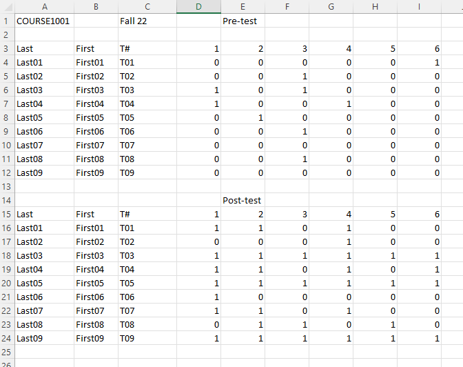
Note that this files contains two DataFrames.

The first is the result of the pretest, which is from row 3 to row 11, with the header row 2.
The second is the result of the posttest, which is from row 15 to row 23, with the header row 14. To read the file, the code is as follows:

import pandas as pd

df_pre = pd.read_excel('assests/datasets/prepost.xlsx',
                       engine='openpyxl',
                       header=2, 
                       nrows=10)
df_pre

	Last	First	T#	1	2	3	4	6	7	9	10	Unnamed: 13
0	Last01	First01	T01	0	0	0	0	1	0	0	0	NaN
1	Last02	First02	T02	0	0	1	0	0	0	1	1	NaN
2	Last03	First03	T03	1	0	1	0	0	0	0	0
3	Last04	First04	T04	1	0	0	1	0	0	0	0	NaN
4	Last05	First05	T05	0	1	0	0	0	0	0	0	NaN
5	Last06	First06	T06	0	0	1	0	0	1	0	1	NaN
6	Last07	First07	T07	0	0	0	0	0	0	0	0	NaN
7	Last08	First08	T08	0	0	1	0	0	0	0	0	NaN
8	Last09	First09	T09	0	0	0	0	0	1	0	1	NaN

df_post = pd.read_excel('assests/datasets/prepost.xlsx',
                        engine='openpyxl',
                        header=14,
                        nrows=10)                      
df_post

	Last	First	T#	1	2	3	4	5	6	7	8	9	10	Unnamed: 13
0	Last01	First01	T01	1	1	0	1	0	0	0	0	1	1	NaN
1	Last02	First02	T02	0	0	0	1	0	0	1	0	0	0	NaN
2	Last03	First03	T03	1	1	1	1	1	1	0	0	1	0	NaN
3	Last04	First04	T04	1	1	0	1	0	1	0	0	1	0	NaN
4	Last05	First05	T05	1	1	1	1	1	1	0	0	0	0	NaN
5	Last06	First06	T06	1	0	0	0	0	0	0	0	0	1	NaN
6	Last07	First07	T07	1	1	0	1	0	0	0	0	0	0	NaN
7	Last08	First08	T08	0	1	1	0	1	0	0	1	1	0	NaN
8	Last09	First09	T09	1	1	1	1	1	1	0	1	0	0	NaN

It seems that the original files have an additional column Unnamed: 13 containing nan values that should be dropped. Then it is not necessary to read it from the original file. Here we could use the argument usecols to select the first 13 columns. We only show the example of pretest result.

df_pre = pd.read_excel('assests/datasets/prepost.xlsx',
                       engine='openpyxl',
                       header=2, 
                       nrows=10,
                       usecols=list(range(13)))
df_pre

	Last	First	T#	1	2	3	4	6	7	9	10
0	Last01	First01	T01	0	0	0	0	1	0	0	0
1	Last02	First02	T02	0	0	1	0	0	0	1	1
2	Last03	First03	T03	1	0	1	0	0	0	0	0
3	Last04	First04	T04	1	0	0	1	0	0	0	0
4	Last05	First05	T05	0	1	0	0	0	0	0	0
5	Last06	First06	T06	0	0	1	0	0	1	0	1
6	Last07	First07	T07	0	0	0	0	0	0	0	0
7	Last08	First08	T08	0	0	1	0	0	0	0	0
8	Last09	First09	T09	0	0	0	0	0	1	0	1

4.6.2 Write files

We will only talk about writing in csv. The function is df.to_csv(). It is straightforward.

The argument index is used to control whether you want to write index into the file. The default is True. If the index doesn’t contain any real information, we usually set it to be False.

4.7 Example: Movies

Below we explore the MovieLens 1M datasets. You may download it from this link. This is a .dat file, and you may use the following code to read it into a DataFrame.

import pandas as pd
mnames = ['movie_id', 'title', 'genres']
movies = pd.read_table('assests/datasets/movies.dat', sep='::',
                       header=None, names=mnames, engine="python",
                       encoding='ISO-8859-1')
movies.head()

	movie_id	title	genres
0	1	Toy Story (1995)	Animation\|Children's\|Comedy
1	2	Jumanji (1995)	Adventure\|Children's\|Fantasy
2	3	Grumpier Old Men (1995)	Comedy\|Romance
3	4	Waiting to Exhale (1995)	Comedy\|Drama
4	5	Father of the Bride Part II (1995)	Comedy

In this example we concentrate on exploring the genres information. We first want to find all genres in this dataset. The idea is:

split each item in the genres column by | to get a list.
go through each item in the genres column, and union all lists together.

This can be done by the map function.

Tips

all_genres = list()
movies['genres'].map(lambda x: all_genres.extend(x.split('|')))

0       None
1       None
2       None
3       None
4       None
        ... 
3878    None
3879    None
3880    None
3881    None
3882    None
Name: genres, Length: 3883, dtype: object

all_genres is the list of all genres (with duplicates).

In the output of the above code you may see many None in each row. This is because the lambda function used in map doesn’t have a return value. However after applying the function to each row, new genres information is added to the list all_genres.

Then we would like to drop all the duplicates to get the list of all unique genres.

Tips

genres = pd.unique(all_genres)
genres

array(['Animation', "Children's", 'Comedy', 'Adventure', 'Fantasy',
       'Romance', 'Drama', 'Action', 'Crime', 'Thriller', 'Horror',
       'Sci-Fi', 'Documentary', 'War', 'Musical', 'Mystery', 'Film-Noir',
       'Western'], dtype=object)

genres is the list of all unique genres.

4.8 Exercises

Many problems are based on [1].

Exercise 4.1 Let df be a DataFrame. Please answer the following questions in a Markdown cell.

What does df[0] do?
What does df[[0]] do?
What does df[0:1] do?

Exercise 4.2 Please use the following code to generate a series ser, and then finish the following tasks.

import pandas as pd
import numpy as np


mylist = list('abcedfghijklmnopqrstuvwxyz')
myarr = np.arange(26)
mydict = dict(zip(mylist, myarr))
ser = pd.Series(mydict)

Convert the series ser into a dataframe df with its index as another column on the dataframe.
Pick the two columns of df and set them into two serieses ser1 and ser2.
Combine two series ser1 and ser2 to form a new dataframe newdf, and name their columns ser1 and ser2.

Exercise 4.3 Consider two serieses ser1 and ser2. You may use the following ser1 and ser2 as an example. The output of each questions below should be a series. You may want to learn the following commands:

import pandas as pd

ser1 = pd.Series([1, 2, 3, 4, 5])
ser2 = pd.Series([4, 5, 6, 7, 8])

Find all the elements from ser1 that are also in ser2.
Find all the elements from ser2 that are also in ser1.
From ser1 remove items present in ser2.
Find the union of ser1 and ser2.
Find the intersection of ser1 and ser2.
Find all the elemetns that are in either ser1 or ser2, but not both.

Exercise 4.4 Consider the following DataFrame.

import pandas as pd

data = pd.DataFrame(np.arange(16).reshape((4, 4)),
                    index=['Ohio', 'Colorado', 'Utah', 'New York'],
                    columns=['one', 'two', 'three', 'four'])

Please select the column two.
Please select the second and the third row.
Please find the rows that the column three value is bigger than 5.
Please find the last row that the column three value is bigger than 5.
Please find the rows that the column three value is bigger than 5, and display the resulted DataFrame with only Colorado and Utah row and four and one columns, in the specified order.

Exercise 4.5 Consider the following Series.

import pandas as pd
import numpy as np
ser = pd.Series(np.take(list('abcdefgh'), np.random.randint(8, size=30)))

Please use pd.Series.value_counts() to calculte the frequency counts of each unique value of the following Series.
Please keep the top 2 most frequent items of ser as it is and replace everything else as Other.

Exercise 4.6 Consider the Series ser:

import pandas as pd
import numpy as np
ser = pd.Series(np.random.randint(1, 10, 7))

Find the positions of numbers that are multiples of 3 from ser.

Exercise 4.7 Compute the mean of weights of each fruit.

import pandas as pd
fruit = pd.Series(np.random.choice(['apple', 'banana', 'carrot'], 10))
weights = pd.Series(np.linspace(1, 10, 10))
df = pd.DataFrame({'fruit': fruit, 'weights': weights})

Exercise 4.8 Consider the following DataFrame.

import pandas as pd
df = pd.read_csv('https://raw.githubusercontent.com/selva86/datasets/master/Cars93_miss.csv')

Check if df has any missing values.
Please count the number of missing values in each column.
Please replace all missing values in Min.Price and Max.Price with their mean respectively.

Exercise 4.9 Get the last two rows of df whose row sum is greater than 100.

import pandas as pd
df = pd.DataFrame(np.random.randint(10, 40, 60).reshape(-1, 4))

Exercise 4.10 The groupby object df_grouped is given below.

import pandas as pd
import numpy as np
df = pd.DataFrame({'fruit': ['apple', 'banana', 'orange'] * 3,
                   'price': np.random.rand(9),
                   'taste': np.random.randint(0, 11, 9)})

df_grouped = df.groupby(['fruit'])

Get the group belonging to apple as a DataFrame.
Find the second largest value of taste for banana.
Compute the mean price for every fruit.

Exercise 4.11 Join df1 and df2 by fruit/pazham and weight/kilo.

df1 = pd.DataFrame({'fruit': ['apple', 'banana', 'orange'] * 3,
                    'weight': ['high', 'medium', 'low'] * 3,
                    'price': np.random.randint(0, 15, 9)})

df2 = pd.DataFrame({'pazham': ['apple', 'orange', 'pine'] * 2,
                    'kilo': ['high', 'low'] * 3,
                    'price': np.random.randint(0, 15, 6)})

Exercise 4.12 Consider the following DataFrame.

import pandas as pd
import numpy as np
df = pd.read_csv('https://raw.githubusercontent.com/selva86/datasets/master/Cars93_miss.csv', usecols=[0,1,2,3,5])

Replace NaN with string missing in columns Manufacturer, Model and Type.
Create an index as a combination of these three columns.

Exercise 4.13 Given the following DataFrame.

import pandas as pd
df = pd.DataFrame({
    'name': ['James', 'Jane', 'Melissa', 'Ed', 'Neil'],
    'age': [30, 40, 32, 67, 43],
    'score': ['90%', '95%', '100%', '82%', '87%'],
    'age_missing_data': [30, 40, 32, 67, None],
    'income':[100000, 80000, 55000, 62000, 120000]
})

Please use .map to create a new column numeric_score whose value is the number version of score.
Please use .apply to create a new column numeric_score whose value is the number version of score.

Exercise 4.14 The following DataFrame is given.

import pandas as pd
df = pd.DataFrame(["STD, City    State",
                   "33, Kolkata    West Bengal",
                   "44, Chennai    Tamil Nadu",
                   "40, Hyderabad    Telengana",
                   "80, Bangalore    Karnataka"],
                   columns=['row'])

Please create a new DataFrame out of df by spliting it into three columns based on , and four spaces. In addition, the column names of the new DataFrame are given by the first row of df.

4.1 Basic pandas

4.1.1 Series and DataFrame

4.1.2 Decorations

4.1.3 Look at the DataFrame

4.2 Indexing

4.2.1 []

4.2.2 .loc[] and .iloc[]

4.2.3 Boolean indexing

4.2.4 .query()

4.2.5 Reindex

4.2.6 Updating data

4.3 Data cleaning

4.3.1 Handling Missing Data

4.3.2 Handling duplicates

4.3.3 Drop data

4.3.4 String Manipulation

4.4 Data Wrangling

4.4.1 Tidy data

4.4.2 Hierarchical indexing

4.4.3 Combining and Merging Datasets

4.5 Data Aggregation and Group Operations

4.5.1 split-apply-combine model

4.5.2 Built-in aggregation functions

4.5.3 Function Application and Mapping

4.5.4 Some examples

4.6 Read and write files

4.6.1 Read files

4.6.2 Write files

4.7 Example: Movies

4.8 Exercises

4.1 Basic `pandas`

4.1.1 `Series` and `DataFrame`

4.1.3 Look at the `DataFrame`

4.2.1 `[]`

4.2.2 `.loc[]` and `.iloc[]`

4.2.4 `.query()`