x <- seq(-4, 4, length=100)
y <- dnorm(x, mean=2, sd=0.5)
plot(x, y, type="l")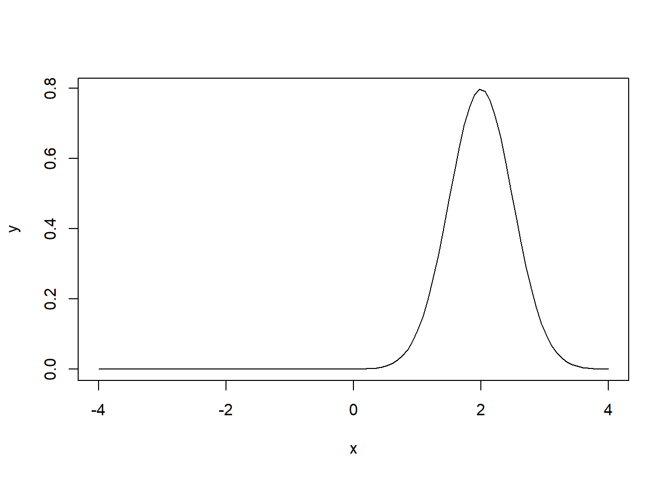
\[ \require{physics} \require{braket} \]
\[ \newcommand{\dl}[1]{{\hspace{#1mu}\mathrm d}} \newcommand{\me}{{\mathrm e}} \newcommand{\argmin}{\operatorname{argmin}} \]
$$
$$
\[ \newcommand{\pdfbinom}{{\tt binom}} \newcommand{\pdfbeta}{{\tt beta}} \newcommand{\pdfpois}{{\tt poisson}} \newcommand{\pdfgamma}{{\tt gamma}} \newcommand{\pdfnormal}{{\tt norm}} \newcommand{\pdfexp}{{\tt expon}} \]
\[ \newcommand{\distbinom}{\operatorname{B}} \newcommand{\distbeta}{\operatorname{Beta}} \newcommand{\distgamma}{\operatorname{Gamma}} \newcommand{\distexp}{\operatorname{Exp}} \newcommand{\distpois}{\operatorname{Poisson}} \newcommand{\distnormal}{\operatorname{\mathcal N}} \newcommand{\distunif}{\operatorname{Unif}} \]
Definition 2.1 (Expectation) \[ \operatorname{E}\mqty[u(X)] = \int_{-\infty}^{\infty}u(x)f(x)\dl3x. \]
Definition 2.2
Proposition 2.1
\[ \begin{split} \operatorname{E}\mqty[ag(X)+bh(X)]&=\int_{-\infty}^{\infty}\mqty[ag(x)+bh(x)]f(x)\dl3x\\ &=a\int_{-\infty}^{\infty}g(x)f(x)\dl3x+b\int_{-\infty}^{\infty}h(x)f(x)\dl3x\\ &=a\operatorname{E}\mqty[g(X)]+b\operatorname{E}\mqty[h(X)]. \end{split} \]
\[ \begin{split} \operatorname{E}\mqty[(X-\mu)^2]&=\operatorname{E}\mqty[\qty(X^2-2\mu X+\mu^2)]=\operatorname{E}(X^2)-2\mu\operatorname{E}(X)+\operatorname{E}(\mu^2)\\ &=\operatorname{E}(X^2)-2\mu\mu+\mu^2=\operatorname{E}(X^2)-\mu^2. \end{split} \]
\[ \begin{split} \operatorname{Var}\mqty[aX]&=\operatorname{E}(a^2X^2)-a^2\mu^2=a^2\qty(\operatorname{E}(X^2)-\mu^2)=a^2\operatorname{Var}(X),\\ \operatorname{Var}\mqty[X+Y]&=\operatorname{E}((X+Y)^2)-(\operatorname{E}(X+Y))^2\\ &=\operatorname{E}(X^2)+\operatorname{E}(Y^2)+2\operatorname{E}(XY)-\operatorname{E}(X)^2-\operatorname{E}(Y)^2-2\operatorname{E}(X)\operatorname{E}(Y)\\ &=\operatorname{Var}(X)+\operatorname{Var}(Y)+2(E(XY)-E(X)E(Y))\\ &=\operatorname{Var}(X)+\operatorname{Var}(Y),\\ \operatorname{Var}\mqty[aX+bY]&=a^2\operatorname{Var}(X)+b^2\operatorname{Var}(Y). \end{split} \]
Assume \(X_1,\ldots, X_n\) i.i.d. with mean \(\mu\) and variance \(\sigma^2\). Then \(\operatorname{Var}(\frac1n\sum X_i)=\sigma^2/n\). This implies that the more samples you pick, the smaller the variance is. This explains why, when possible, we want a large sample size. Note that we don’t specify any concrete distribution in this remark. This is related to estimation, which will be discussed in detail later.
R has built-in random variables with different distributions. The naming convention is a prefix d-, p-, q- and r- together with the name of distribution.
d-: density function of the given distribution;p-: cumulative density function of the given distribution;q-: quantile function of the given distribution (which is the inverse of p- function);r-: random sampling from the given distribution.Example 2.1 (Normal distribution)
x <- seq(-4, 4, length=100)
y <- dnorm(x, mean=2, sd=0.5)
plot(x, y, type="l")
x <- seq(-4, 4, length=100)
y <- pnorm(x, mean=2, sd=0.5)
plot(x, y, type="l")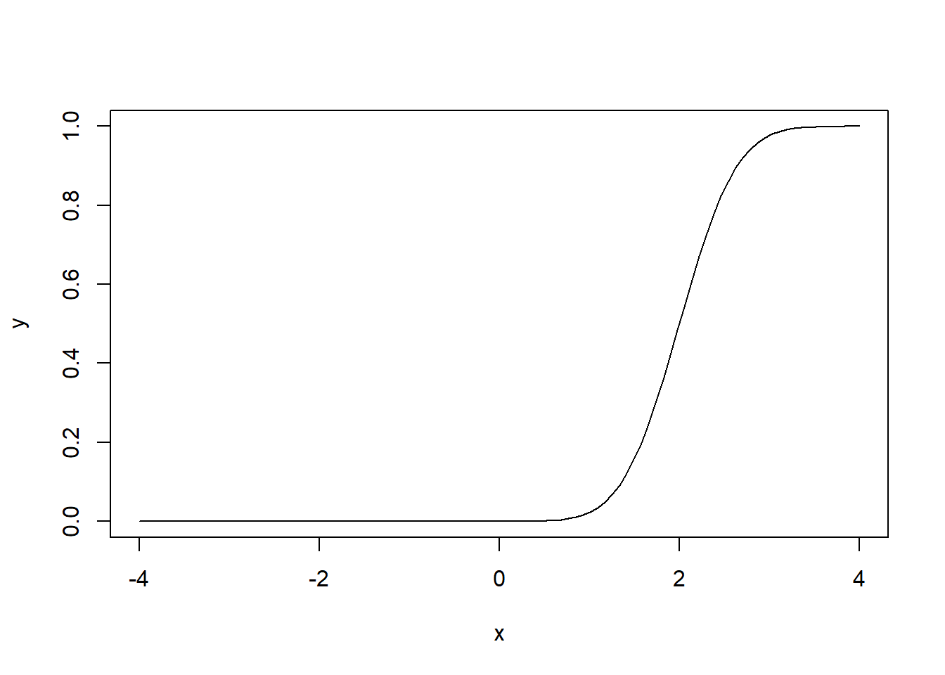
qnorm(0.025)[1] -1.959964qnorm(0.5)[1] 0qnorm(0.975)[1] 1.959964rnorm(10) [1] -2.1520996 0.8154634 1.3972201 -0.3558444 0.9952280 -0.8886770
[7] 1.1540617 0.3979143 -0.3107844 -0.8612821Assuming we have two random variables \(X\) and \(Y\), and we have two sets of realizations \(x_1,\ldots, x_n\) and \(y_1,\ldots, y_n\).
The sum of squares and cross-products are defined as
where \(\bar x\) and \(\bar y\) are sample mean. Note that if we normalize these quantities by \(n-1\), we will get the usual unbiased sample varaince and covariance.
Definition 2.3 (Covariance and sample covariance)
Definition 2.4 (Pearson correlation coefficient \(r\)) \[ r=\operatorname{cor}(x,y)=\frac{SS_{xy}}{\sqrt{{SS_{xx}SS_{yy}}}}. \]
Theorem 2.1 (Properties of Correlation)
The Pearson correlation coefficient is used to measure the correlation of the two variables. If the relation is more closely stick to a straight line, the relation is stronger, and the resulted \(r\) will be bigger. If \(r=1\), \(X\) and \(Y\) will have a perfectly linear relation. This is not the same as the slope.
Example 2.2 Let \(x_i=i\) and \(y_i=0.001x_i\). Then the slope is \(0.001\) and the \(r=1\). We may add a small noise to it so \(y_i=0.001x_i+\varepsilon_i\) while \(\varepsilon_i\sim N(0,0.001)\). Then the slope is \(0.001\) but \(r\) is still close to \(1\).
x <- seq(1, 100)
y <- 0.001 * x + rnorm(100, 0, 1e-3)
plot(x, y)
abline(0, 0.001, col='red')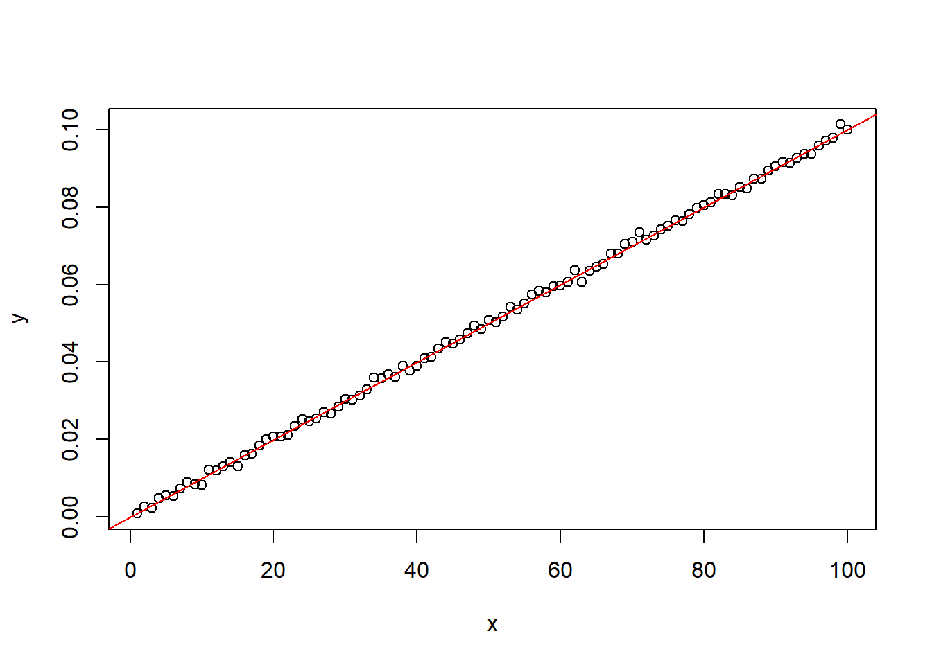
cor(x, y)[1] 0.9995071Independence is the relation between two random variables.
Definition 2.5 (Independence) Random variables \(X\) and \(𝑌\) are said to be independent if their joint distribution factorizes into the product of their marginal distributions. That is, for all \(x\), \(y\) \[ F_{X,Y}(x,y)=F_X(x)F_Y(y). \]
If a joint density exists, this is equivalently written as
\[ f_{X,Y}(x,y)=f_X(x)f_Y(y). \]
It is equivalent to say that for all measurable functions \(g\) and \(h\),
\[ \operatorname{E}[g(X)h(Y)]=\operatorname{E}[g(X)]\operatorname{E}[h(Y)]. \]
Independence concerns the entire joint distribution, not just a summary statistic. Specifically, it cannot be derived from \(\operatorname{Cov}\) and \(\operatorname{cor}\).
Theorem 2.2 If \(X\) and \(Y\) are independent, then \(\operatorname{Cov}(X,Y)=0\) and \(\operatorname{cor}(X,Y)=0\). The converse is not true in general.
\(\operatorname{Cov}(X,Y)=0\) (equivalently, \(\operatorname{cor}(X,Y)=0\)) means that \(X\) and \(Y\) have no positive or negative linear relationship. However, this does not imply that \(X\) and \(Y\) are unrelated; they may still exhibit a nonlinear dependence.
Example 2.3
x <- seq(-10, 10)
y <- abs(x)
cov(x, y)
[1] 0cor(x, y)[1] 0plot(x, y)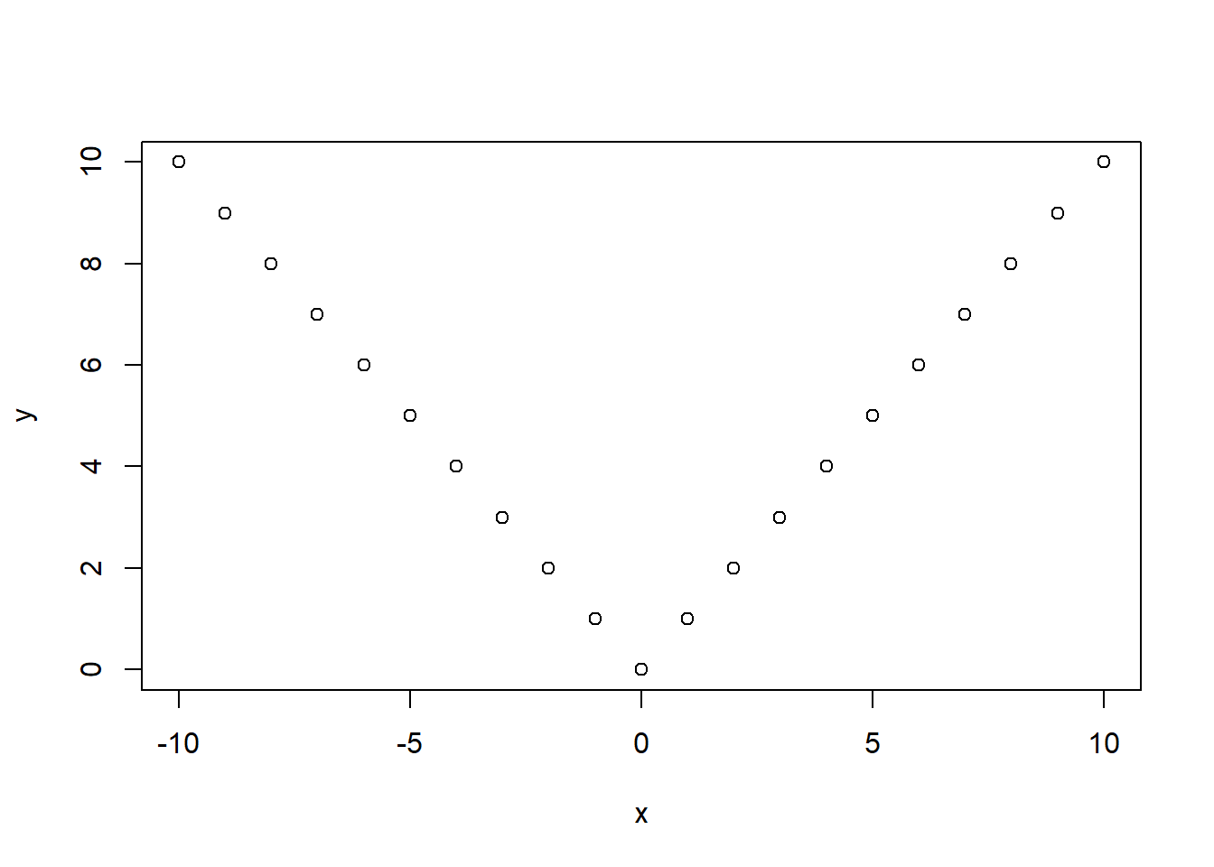
They are not independent because \(y\) is literally defined as a function of \(x\). But their covariance and correlation are \(0\)s.
Theorem 2.3 (Normal Sample Mean–Variance) Let \(X_1,\ldots,X_n\sim N(\mu,\sigma^2)\) i.i.d. Define
Then
The complete proof is lengthy and out of scope of the course. Please refer to [1] for details.
Theorem 2.4 (Student’s t-Distribution [1]) Let
Then \[ T=\frac{Z}{\sqrt{U/\nu}} \] has a Student’s t-distribution with \(\nu\) degrees of freedom: \(T\sim t_{\nu}\).
These two theorems are usually used together. Let \(X_1,\ldots,X_n\sim N(\mu,\sigma^2)\) i.i.d. Then
Therefore
So \[ T=\frac{Z}{\sqrt{U/\nu}}=\frac{\frac1{\sigma/\sqrt n}(\bar X-\mu)}{\sqrt{\frac{(n-1)s^2}{\sigma^2}/(n-1)}}=\frac{\bar X-\mu}{s/\sqrt n}\sim t_{n-1}. \]
In other words, if we standardize the sample mean using the sample standard deviation, we obtain a statistic that follows a t-distribution. This result is mainly used in the t-test.
The normal distribution and the t-distribution are both bell-shaped and symmetric. When the sample size is large (typically (n > 30)), the t-distribution becomes very similar to the standard normal distribution, so the normal approximation is usually acceptable. When the sample size is small, however, the t-distribution has noticeably heavier tails, and it is better to use the t-distribution directly for inference.