library(MASS)
data(Boston)11 Example: Boston Housing part 2
We continue to look at the Boston Housing price dataset.
Recall that
| Variable | Description | Type |
|---|---|---|
crim |
Per capita crime rate by town | Numerical, continuous |
zn |
Proportion of residential land zoned for lots over 25,000 sq.ft. | Numerical, continuous |
indus |
Proportion of non-retail business acres per town | Numerical, continuous |
chas |
Charles River dummy variable (1 if tract bounds river; 0 otherwise) | Categorical, nominal |
nox |
Nitrogen oxides concentration (parts per 10 million) | Numerical, continuous |
rm |
Average number of rooms per dwelling | Numerical, continuous |
age |
Proportion of owner-occupied units built prior to 1940 | Numerical, continuous |
dis |
Weighted mean distance to five Boston employment centers | Numerical, continuous |
rad |
Index of accessibility to radial highways (larger = better accessibility) | Categorical, ordinal |
tax |
Full-value property-tax rate per $10,000 | Numerical, continuous |
ptratio |
Pupil–teacher ratio by town | Numerical, continuous |
black |
\(1000(B_k - 0.63)^2\), where \(B_k\) is the proportion of Black residents | Numerical, continuous |
lstat |
Percentage of lower-status population | Numerical, continuous |
medv |
Median value of owner-occupied homes (in $1,000s) | Numerical, continuous |
We need to change chas and rad to be factors.
Boston$chas <- factor(Boston$chas)
Boston$rad <- factor(Boston$rad)
11.1 With all predictors
We start from the full model with all predictors.
fit.full <- lm(medv ~ ., data=Boston)
anova_alt(fit.full)
Analysis of Variance Table
Df SS MS F P
Source 20 32032 1601.58 72.698 8.2948e-132
Error 485 10685 22.03
Total 505 42716 All variables as a group are significant.
Now we consider building a model with part of the predictors. We have 13 independent variables to choose. Should all the predictors be included in the model? Or use only a couple of them? Which ones should be in the model? We will decide by using variable selection procedures, which is discussed in the next unit.
By using variable selection procedures, we could identify the most important predictors. For now, let’s say, we are going to fit models with 5 predictors chosen: lstat, rm, dis, ptratio, chas.
Boston_5_pred <- Boston[, c("lstat", "rm", "dis", "ptratio","chas", "medv")]First, we model medv (\(y\)) as a function of the lower status of the population lstat (\(x_1\)), average number of rooms rm (\(x_2\)), distance to Boston employment centres dis (\(x_3\)), pupil-teacher ratio ptratio (\(x_4\)), and if tract bounds river chas (\(x_5\)).
fit0 <- lm(medv ~ lstat + rm + dis + ptratio + chas, data = Boston_5_pred)
summary(fit0)
Call:
lm(formula = medv ~ lstat + rm + dis + ptratio + chas, data = Boston_5_pred)

Residuals:
     Min       1Q   Median       3Q      Max
-17.9355  -2.9712  -0.6246   1.8183  27.3931

Coefficients:
            Estimate Std. Error t value Pr(>|t|)
(Intercept) 23.46692    4.05271   5.790 1.24e-08 ***
lstat       -0.65845    0.04637 -14.198  < 2e-16 ***
rm           4.17966    0.42016   9.948  < 2e-16 ***
dis         -0.49227    0.12715  -3.871 0.000123 ***
ptratio     -0.93220    0.11569  -8.058 5.75e-15 ***
chas1        2.92247    0.90989   3.212 0.001404 **
---
Signif. codes:  0 '***' 0.001 '**' 0.01 '*' 0.05 '.' 0.1 ' ' 1

Residual standard error: 5.091 on 500 degrees of freedom
Multiple R-squared:  0.6966,    Adjusted R-squared:  0.6935
F-statistic: 229.6 on 5 and 500 DF, p-value: < 2.2e-16anova_alt(fit0)Analysis of Variance Table
Df SS MS F P
Source 5 29755 5951.0 229.56 5.7196e-127
Error 500 12961 25.9
Total 505 42716 Since the p-value from the ANOVA table is small, these 5 variables as a group are significantly related to medv.
11.2 Is chas significant in the above model?
To answer this question, we simply look at the summary table of fit0. From the table all 5 variables are significant. We would like to discuss chas in details since it is qualitative.
coef(summary(fit0))['chas1', ] Estimate Std. Error t value Pr(>|t|)
2.922471289 0.909893844 3.211881593 0.001403636 From the output above, we could find on average, when controlling all other variables, the expected value of the median value of a house is $2922.5 higher for the houses tract bounds river than those not.
We could also perfer a hypothesis test as follows:
- \(H_0:\)
chasis not a significant predictor in the 5 variable model. - \(H_a:\)
chasis a significant predictor in the 5 variable model.
Since p-value = 0.001403636 \(<\alpha=\) 0.05, the null hypothesis is rejected. We conclude that chas is a significant predictor in the 5 variable model.
Click to expand if you are interested in testing chas individually.
We fit the regression model with medv as the \(y\) and chas as the independent variable \(x_5\). Note that, chas is a dummy variable with 2 options. Therefore not tract bounds river (chas=0) is chosen as the base level.
fit_chas<-lm(medv ~ chas, data = Boston_5_pred)
summary(fit_chas)
Call:
lm(formula = medv ~ chas, data = Boston_5_pred)

Residuals:
    Min      1Q  Median      3Q     Max
-17.094  -5.894  -1.417   2.856  27.906

Coefficients:
            Estimate Std. Error t value Pr(>|t|)
(Intercept)  22.0938     0.4176  52.902  < 2e-16 ***
chas1         6.3462     1.5880   3.996 7.39e-05 ***
---
Signif. codes:  0 '***' 0.001 '**' 0.01 '*' 0.05 '.' 0.1 ' ' 1

Residual standard error: 9.064 on 504 degrees of freedom
Multiple R-squared:  0.03072,   Adjusted R-squared:  0.02879
F-statistic: 15.97 on 1 and 504 DF, p-value: 7.391e-05anova_alt(fit_chas)Analysis of Variance Table
Df SS MS F P
Source 1 1312 1312.08 15.972 7.3906e-05
Error 504 41404 82.15
Total 505 42716 From the output above, we could find on average, the expected value of the median value of a house is $6346 higher for the houses tract bounds river than those not.
We could also perfer a hypothesis test as follows:
- \(H_0:\)
chasis not a significant predictor. - \(H_a:\)
chasis a significant predictor.
chas is a significant predictor. However, on the other hand, the coefficient of determination \(r^2=0.03\), which is quite small value. In other word, in addition to chas, we need more predictors in the model.
11.3 The relationship between lstat and medv
In SLR, we fitted straight-line model to relate medv (\(y\)) and lstat (\(x_1\)).
plot(Boston$lstat, Boston$medv)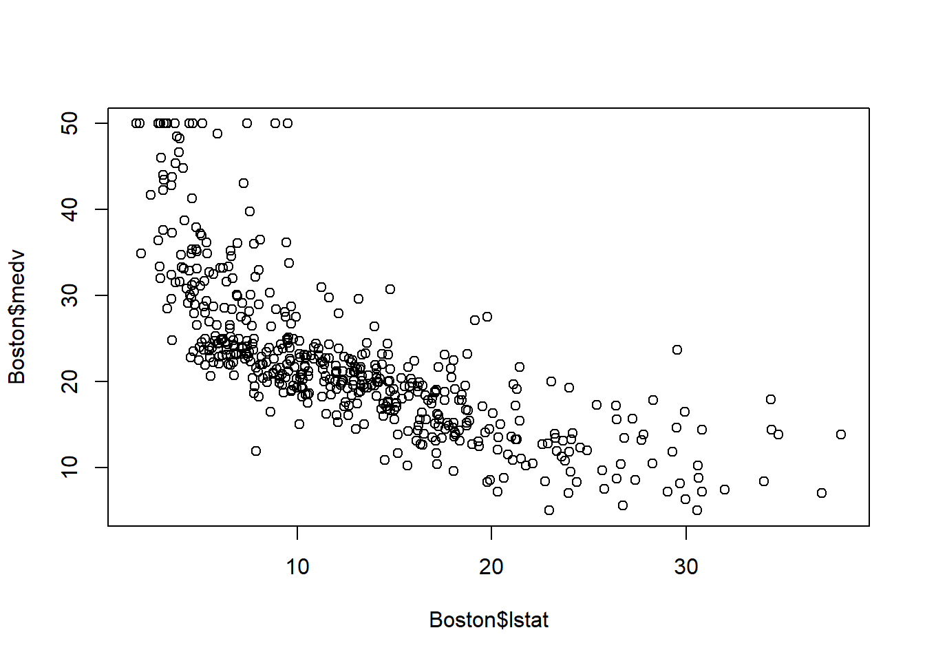
fit_lstat <- lm(medv ~ lstat, data = Boston_5_pred)The scatterplot shows curvilinear relationship, which suggests a curivilinear model might be a better fit. We will fit the curvilinear model \(y=\beta_0+\beta_1 x_1+\beta_2 x_1^2+\varepsilon\).
fit_quad <- lm(medv ~ lstat + I(lstat^2), data = Boston_5_pred)
summary(fit_quad)
Call:
lm(formula = medv ~ lstat + I(lstat^2), data = Boston_5_pred)

Residuals:
     Min       1Q   Median       3Q      Max
-15.2834  -3.8313  -0.5295   2.3095  25.4148

Coefficients:
             Estimate Std. Error t value Pr(>|t|)
(Intercept) 42.862007   0.872084   49.15   <2e-16 ***
lstat       -2.332821   0.123803  -18.84   <2e-16 ***
I(lstat^2)   0.043547   0.003745   11.63   <2e-16 ***
---
Signif. codes:  0 '***' 0.001 '**' 0.01 '*' 0.05 '.' 0.1 ' ' 1

Residual standard error: 5.524 on 503 degrees of freedom
Multiple R-squared:  0.6407,    Adjusted R-squared:  0.6393
F-statistic: 448.5 on 2 and 503 DF, p-value: < 2.2e-16anova_alt(fit_quad)Analysis of Variance Table
Df SS MS F P
Source 2 27369 13684.5 448.51 1.5572e-112
Error 503 15347 30.5
Total 505 42716 First, we test the overall significance of this curvilinear model.
- \(H_0: \beta_1=\beta_2=0\)
- \(H_a:\) At least one of the \(\beta\)’s \(\neq 0\)
Since the p-value is almost 0, which is less than \(\alpha=0.05\), we reject \(H_0\) and conclude the curvilinear model is adequate.
In order to identify whether the curvilinear term lstat\(^2\) should be kept in the model, we could run the \(t\)-test, or partial \(F\)-test. Since there is only one additional factor (i.e. lstat\(^2\)) is considered here, these two tests are equivalent.
anova(fit_lstat, fit_quad)Analysis of Variance Table
Model 1: medv ~ lstat
Model 2: medv ~ lstat + I(lstat^2)
Res.Df RSS Df Sum of Sq F Pr(>F)
1 504 19472
2 503 15347 1 4125.1 135.2 < 2.2e-16 ***
---
Signif. codes: 0 '***' 0.001 '**' 0.01 '*' 0.05 '.' 0.1 ' ' 1\(H_0: y=\beta_0+\beta_1 x\) (Reduced Model)
\(H_a:y=\beta_0+\beta_1 x +\beta_2 x^2\) (Complete Model)
Since the \(p\)-value =7.63e-28 \(<\alpha\), we reject \(H_0\) and conclude the complete model is preferred. Therefore, medv and lstat are related in a curvilinear way, with upward curvature (as \(\beta_2>0\)).
Caution
This analysis serves only as a preliminary check. Any candidate quadratic or interaction term should be assessed again in the full multiple regression model, since its significance may change after adjusting for the other predictors. The same applies to the next two sections.
11.4 Interaction between rm and dis
An analyst hypothesizes that the effect of distance to Boston employment centres on house price will be greater when there are more room numbers. To test this hypothesis, we will need to run an interaction model for \(E(y)\) as a function of rm (\(x_2\)), dis(\(x_3\)), and rm:dis (\(x_2x_3\)).
fit_interaction <- lm(medv ~ rm * dis, data = Boston_5_pred)
summary(fit_interaction)
Call:
lm(formula = medv ~ rm * dis, data = Boston_5_pred)

Residuals:
    Min      1Q  Median      3Q     Max
-18.423  -3.276   0.104   2.831  38.061

Coefficients:
            Estimate Std. Error t value Pr(>|t|)
(Intercept) -15.2533     4.8953  -3.116  0.00194 **
rm            5.7020     0.7851   7.263 1.45e-12 ***
dis          -5.7579     1.3500  -4.265 2.39e-05 ***
rm:dis        0.9855     0.2119   4.652 4.22e-06 ***
---
Signif. codes:  0 '***' 0.001 '**' 0.01 '*' 0.05 '.' 0.1 ' ' 1

Residual standard error: 6.415 on 502 degrees of freedom
Multiple R-squared:  0.5164,    Adjusted R-squared:  0.5135
F-statistic: 178.7 on 3 and 502 DF, p-value: < 2.2e-16anova_alt(fit_interaction)Analysis of Variance Table
Df SS MS F P
Source 3 22057 7352.5 178.66 8.3739e-79
Error 502 20659 41.2
Total 505 42716 - \(H_0\): There is no significant interaction between
rmanddis. - \(H_a:\) There is a significant interaction between
rmanddis.
From the p-value = 0.0000042 \(<\alpha=.05\) for rm:dis in the summary table, we conclude there is a significant interaction between rm and dis. This suggests that distance from Boston employment centres and number of rooms interact positively in their association with median house price.
11.5 Interaction between chas and dis
As an additional illustration, we may also examine whether the effect of distance to Boston employment centres depends on whether the tract bounds the Charles River. Compared with the earlier cases of lstat^2 and rm:dis, this interaction is more exploratory and is included mainly to demonstrate how an additional interaction term can be tested.
To investigate this, we fit a model with chas, dis, and their interaction chas:dis.
fit_interaction2 <- lm(medv ~ chas * dis, data = Boston_5_pred)
summary(fit_interaction2)
Call:
lm(formula = medv ~ chas * dis, data = Boston_5_pred)

Residuals:
    Min      1Q  Median      3Q     Max
-14.291  -5.660  -1.572   2.513  31.089

Coefficients:
            Estimate Std. Error t value Pr(>|t|)
(Intercept)  17.5238     0.8279  21.166  < 2e-16 ***
chas1         8.2399     3.9944   2.063   0.0396 *
dis           1.1864     0.1878   6.317 5.89e-10 ***
chas1:dis    -0.3031     1.2088  -0.251   0.8021
---
Signif. codes:  0 '***' 0.001 '**' 0.01 '*' 0.05 '.' 0.1 ' ' 1

Residual standard error: 8.737 on 502 degrees of freedom
Multiple R-squared:  0.103, Adjusted R-squared:  0.09763
F-statistic: 19.21 on 3 and 502 DF, p-value: 8.287e-12anova_alt(fit_interaction2)Analysis of Variance Table
Df SS MS F P
Source 3 4399 1466.49 19.213 8.2873e-12
Error 502 38317 76.33
Total 505 42716 - \(H_0\): There is no significant interaction between
chasanddis. - \(H_a:\) There is a significant interaction between
chasanddis.
From the p-value = 0.8021 \(>\alpha=.05\) for chas:dis in the summary table, we fail to find sufficient evidence of a significant interaction between chas and dis. This suggests that the interaction is not strongly supported at the preliminary stage.
Note
This smaller-model test is part of a preliminary screening step. Its purpose is to identify candidate higher-order/interaction terms before constructing the fuller multiple regression model. If a term is not significant and lacks strong theoretical motivation, it may be dropped at this stage. However, a term that is of substantive interest may still be carried forward and reassessed in the full model, since its significance can change after adjusting for other predictors.
In this example, we retain chas:dis temporarily for illustration and make the final decision later in the fuller model.
11.6 Put things together
Based on the preliminary analyses above, the quadratic term I(lstat^2) and the interaction term rm:dis appear to be promising candidates for the final model. We also include chas:dis temporarily as an exploratory interaction so that its contribution can be reassessed in the fuller multiple regression setting.
Starting from the 5-predictor main-effects model, we next fit a larger model that includes the candidate quadratic and interaction terms under consideration. Here, medv (\(y\)) is modeled using lstat (\(x_1\)), rm (\(x_2\)), dis (\(x_3\)), ptratio (\(x_4\)), and chas (\(x_5\)). \[
y=\beta_0+\beta_1x_1+\beta_2x_2+\beta_3x_3+\beta_4x_4+\beta_5x_5+\beta_6x_1^2+\beta_7x_2x_3+\beta_8x_3x_5+\varepsilon.
\]
fit0 <- lm(medv ~ lstat + rm + dis + ptratio + chas, data = Boston_5_pred)
fit_final0 <- lm(medv ~ lstat + rm + dis + ptratio + chas + I(lstat^2) + rm:dis + chas:dis, data = Boston_5_pred)

summary(fit_final0)
Call:
lm(formula = medv ~ lstat + rm + dis + ptratio + chas + I(lstat^2) +
    rm:dis + chas:dis, data = Boston_5_pred)

Residuals:
     Min       1Q   Median       3Q      Max
-17.8725  -2.8131  -0.4792   2.3980  25.7657

Coefficients:
             Estimate Std. Error t value Pr(>|t|)
(Intercept) 39.120944   4.596990   8.510  < 2e-16 ***
lstat       -1.768398   0.128522 -13.759  < 2e-16 ***
rm           2.301479   0.622749   3.696 0.000244 ***
dis         -2.976134   1.051700  -2.830 0.004846 **
ptratio     -0.714222   0.106117  -6.730 4.67e-11 ***
chas1        2.743745   2.130889   1.288 0.198482
I(lstat^2)   0.031996   0.003538   9.045  < 2e-16 ***
rm:dis       0.366163   0.166298   2.202 0.028135 *
dis:chas1    0.069681   0.643259   0.108 0.913782
---
Signif. codes:  0 '***' 0.001 '**' 0.01 '*' 0.05 '.' 0.1 ' ' 1

Residual standard error: 4.586 on 497 degrees of freedom
Multiple R-squared:  0.7553,    Adjusted R-squared:  0.7514
F-statistic: 191.8 on 8 and 497 DF, p-value: < 2.2e-16anova_alt(fit_final0)Analysis of Variance Table
Df SS MS F P
Source 8 32266 4033.2 191.81 1.2854e-146
Error 497 10451 21.0
Total 505 42716 From the summary table, the interaction term chas:dis is not significant. This agrees with the earlier preliminary analysis. To formally assess whether this interaction should remain in the model, we compare the full model with a reduced model that excludes chas:dis.
fit_chasdis <- lm(medv ~ lstat + rm + dis + ptratio + chas + I(lstat^2) + rm:dis, data = Boston_5_pred)
anova(fit_chasdis, fit_final0)
Analysis of Variance Table
Model 1: medv ~ lstat + rm + dis + ptratio + chas + I(lstat^2) + rm:dis
Model 2: medv ~ lstat + rm + dis + ptratio + chas + I(lstat^2) + rm:dis +
chas:dis
Res.Df RSS Df Sum of Sq F Pr(>F)
1 498 10451
2 497 10451 1 0.24674 0.0117 0.9138Since the p-value is not significant, we do not find sufficient evidence that chas:dis improves the model, so we remove it. Then the updated full model is \[
y=\beta_0+\beta_1x_1+\beta_2x_2+\beta_3x_3+\beta_4x_4+\beta_5x_5+\beta_6x_1^2+\beta_7x_2x_3+\varepsilon.
\]
fit_final1 <- lm(medv ~ lstat + rm + dis + ptratio + chas + I(lstat^2) + rm:dis, data = Boston_5_pred)Next, we assess whether the quadratic term I(lstat^2) should remain in the model by comparing the reduced model without I(lstat^2) to the model that includes it.
fit_nolstat2 <- lm(medv ~ lstat + rm + dis + ptratio + chas + rm:dis, data = Boston_5_pred)
anova(fit_nolstat2, fit_final1)
Analysis of Variance Table
Model 1: medv ~ lstat + rm + dis + ptratio + chas + rm:dis
Model 2: medv ~ lstat + rm + dis + ptratio + chas + I(lstat^2) + rm:dis
Res.Df RSS Df Sum of Sq F Pr(>F)
1 499 12176
2 498 10451 1 1724.7 82.185 < 2.2e-16 ***
---
Signif. codes: 0 '***' 0.001 '**' 0.01 '*' 0.05 '.' 0.1 ' ' 1Since the p-value is small, the quadratic term I(lstat^2) is significant and should be retained.
We then assess the interaction term rm:dis in the same way.
fit_normdis <- lm(medv ~ lstat + rm + dis + ptratio + chas + I(lstat^2), data = Boston_5_pred)
anova(fit_normdis, fit_final1)
Analysis of Variance Table
Model 1: medv ~ lstat + rm + dis + ptratio + chas + I(lstat^2)
Model 2: medv ~ lstat + rm + dis + ptratio + chas + I(lstat^2) + rm:dis
Res.Df RSS Df Sum of Sq F Pr(>F)
1 499 10556
2 498 10451 1 104.92 4.9996 0.02579 *
---
Signif. codes: 0 '***' 0.001 '**' 0.01 '*' 0.05 '.' 0.1 ' ' 1Since the p-value is small, the interaction term rm:dis is significant and should also be retained.
Therefore, the final model is \[ y=\beta_0+\beta_1x_1+\beta_2x_2+\beta_3x_3+\beta_4x_4+\beta_5x_5+\beta_6x_1^2+\beta_7x_2x_3+\varepsilon. \]
fit_final1 <- lm(medv ~ lstat + rm + dis + ptratio + chas + I(lstat^2) + rm:dis, data = Boston_5_pred)
summary(fit_final1)
Call:
lm(formula = medv ~ lstat + rm + dis + ptratio + chas + I(lstat^2) +
    rm:dis, data = Boston_5_pred)

Residuals:
     Min       1Q   Median       3Q      Max
-17.9467  -2.8138  -0.4877   2.3946  25.7730

Coefficients:
             Estimate Std. Error t value Pr(>|t|)
(Intercept) 39.117492   4.592316   8.518  < 2e-16 ***
lstat       -1.767141   0.127871 -13.820  < 2e-16 ***
rm           2.298469   0.621511   3.698 0.000241 ***
dis         -2.988347   1.044602  -2.861 0.004404 **
ptratio     -0.714084   0.106004  -6.736  4.5e-11 ***
chas1        2.956808   0.818973   3.610 0.000337 ***
I(lstat^2)   0.031971   0.003527   9.066  < 2e-16 ***
rm:dis       0.368454   0.164783   2.236 0.025795 *
---
Signif. codes:  0 '***' 0.001 '**' 0.01 '*' 0.05 '.' 0.1 ' ' 1

Residual standard error: 4.581 on 498 degrees of freedom
Multiple R-squared:  0.7553,    Adjusted R-squared:  0.7519
F-statistic: 219.6 on 7 and 498 DF,  p-value: < 2.2e-16
In the final model, all retained terms are significant. The adjusted \(R^2\) is 0.7519, indicating that this model explains a substantial proportion of the variability in medv among the models considered here.
11.7 Utilizing ANOVA tables
In this example, ANOVA tables can be used in several different ways during the model-building process. The choice of Type I, Type II, or Type III ANOVA depends on the question being asked.
11.7.1 Type I ANOVA
Type I ANOVA is the default ANOVA table produced by anova(lm(...)). It tests terms sequentially in the order they appear in the model. In this example, Type I ANOVA is more naturally used during the model-building phase, since it evaluates terms sequentially in the order they are added to the model. This makes it useful for illustrating how much additional variation is explained as new terms are introduced. However, because Type I ANOVA depends on the order of the terms, it is not the best choice for making the final decision about which terms should remain in the model.
11.7.2 Type II ANOVA
Type II ANOVA tests each term after adjusting for the other relevant lower-order terms. It is often a good choice when the model follows the hierarchy principle.
library(car)Loading required package: carDataAnova(fit_final1, type = 2)Anova Table (Type II tests)
Response: medv
Sum Sq Df F value Pr(>F)
lstat 4008.0 1 190.9859 < 2.2e-16 ***
rm 1624.7 1 77.4193 < 2.2e-16 ***
dis 699.0 1 33.3100 1.383e-08 ***
ptratio 952.3 1 45.3785 4.495e-11 ***
chas 273.5 1 13.0349 0.0003367 ***
I(lstat^2) 1724.7 1 82.1853 < 2.2e-16 ***
rm:dis 104.9 1 4.9996 0.0257947 *
Residuals 10450.9 498
---
Signif. codes: 0 '***' 0.001 '**' 0.01 '*' 0.05 '.' 0.1 ' ' 1In this example, Type II ANOVA is mainly useful after we have selected the final model. It gives one table that summarizes whether each retained term still makes a contribution to the model.
Note that summary(fit_final1) gives individual coefficient \(t\)-tests, while the Type II ANOVA table gives term-wise \(F\)-tests. In our final model, each retained term has one degree of freedom, so these two summaries lead to essentially the same conclusions.
Therefore, for this example, the Type II ANOVA table can be used as a convenient alternative summary of term significance in the final selected model.
11.7.3 Type III ANOVA
Type III ANOVA tests each term after adjusting for all other terms in the full model.
library(car)
Anova(fit_final0, type = 3)
Anova Table (Type III tests)
Response: medv
Sum Sq Df F value Pr(>F)
(Intercept) 1522.9 1 72.4222 < 2.2e-16 ***
lstat 3981.0 1 189.3235 < 2.2e-16 ***
rm 287.2 1 13.6580 0.0002437 ***
dis 168.4 1 8.0079 0.0048457 **
ptratio 952.5 1 45.2994 4.674e-11 ***
chas 34.9 1 1.6579 0.1984825
I(lstat^2) 1720.2 1 81.8079 < 2.2e-16 ***
rm:dis 101.9 1 4.8481 0.0281348 *
dis:chas 0.2 1 0.0117 0.9137815
Residuals 10450.7 497
---
Signif. codes: 0 '***' 0.001 '**' 0.01 '*' 0.05 '.' 0.1 ' ' 1In this example, Type III ANOVA is mainly useful for the larger model fit_final0, where several candidate higher-order and interaction terms are included at the same time. It provides a quick way to check whether higher-order terms such as chas:dis, I(lstat^2), and rm:dis remain significant after adjusting for all other terms in that model.
However, Type III ANOVA is not used here as the sole basis for removing terms. To formally decide whether a candidate term should be removed, we still use the corresponding nested model comparison. In addition, Type III ANOVA is less helpful for interpreting lower-order terms, since once higher-order terms are included, the corresponding main effects become harder to interpret.
Therefore, in this example, Type III ANOVA is best viewed as a reference table for the larger candidate model, while the nested model comparisons remain more directly tied to our model-building process.
11.8 Residual analysis
Finally we briefly examine the residuals of the final model using a residual plot.
plot(fitted(fit_final1), resid(fit_final1))
abline(h = 0, col = "red")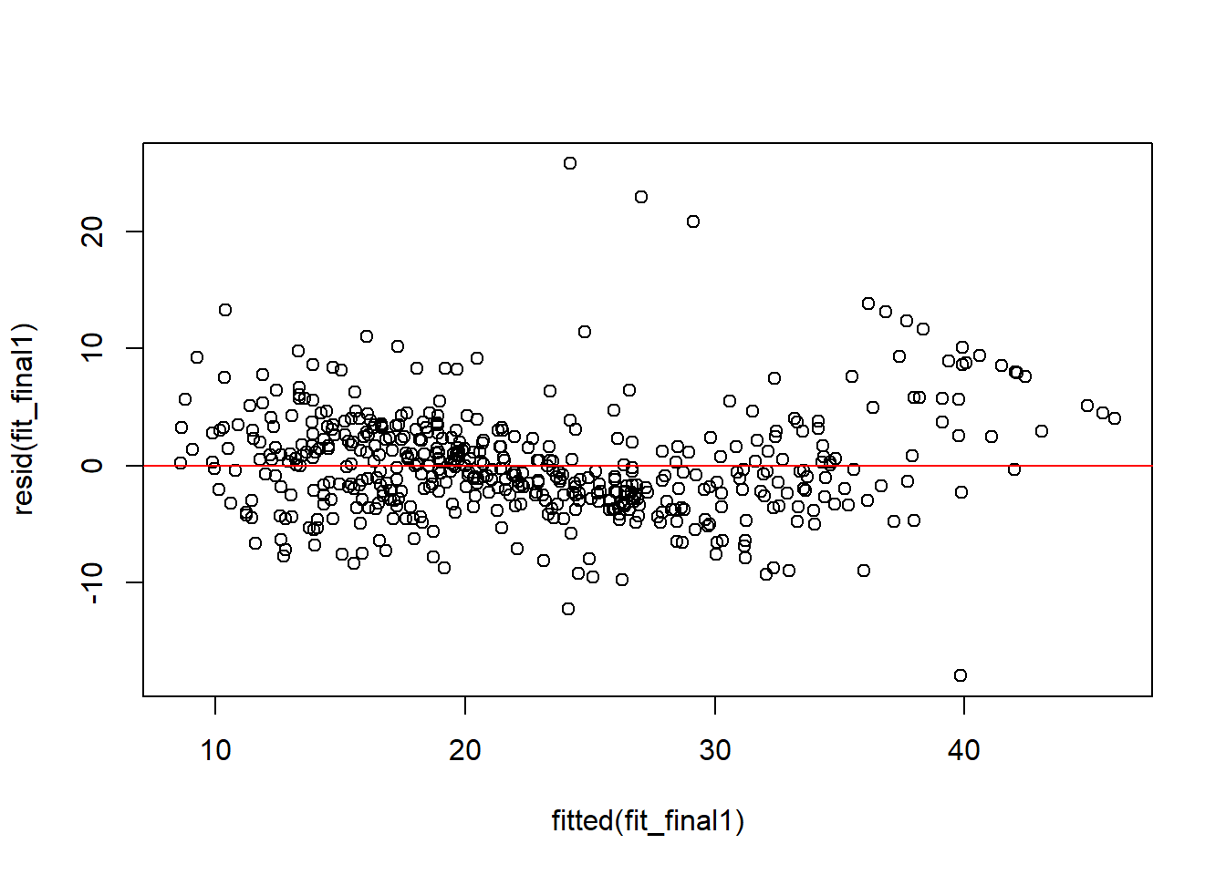
Compared with the residual plot Figure 7.1 from the simple linear regression model, this one shows less obvious structure. This suggests that the final multiple regression model gives a better fit, although the assumptions are still not perfect.
We will formally talk about residual analysis and variable selection in the next unit.