14  Example: Boston Housing dataset full walkthrough

In the previous section we talk about our main tools to handle the Boston dataset. In this section we display how to explore the dataset from scratch.

Variable Description Type
crim Per capita crime rate by town Numerical, continuous
zn Proportion of residential land zoned for lots over 25,000 sq.ft. Numerical, continuous
indus Proportion of non-retail business acres per town Numerical, continuous
chas Charles River dummy variable (1 if tract bounds river; 0 otherwise) Categorical, nominal
nox Nitrogen oxides concentration (parts per 10 million) Numerical, continuous
rm Average number of rooms per dwelling Numerical, continuous
age Proportion of owner-occupied units built prior to 1940 Numerical, continuous
dis Weighted mean distance to five Boston employment centers Numerical, continuous
rad Index of accessibility to radial highways (larger = better accessibility) Categorical, ordinal
tax Full-value property-tax rate per $10,000 Numerical, continuous
ptratio Pupil–teacher ratio by town Numerical, continuous
black \(1000(B_k - 0.63)^2\), where \(B_k\) is the proportion of Black residents Numerical, continuous
lstat Percentage of lower-status population Numerical, continuous
medv Median value of owner-occupied homes (in $1,000s) Numerical, continuous

14.1 Step 1: Understand the Data

Before touching lm(), the first step is always exploratory data analysis (EDA).

library(MASS)
library(car)
data(Boston)

Boston$chas <- factor(Boston$chas)
Boston$rad <- factor(Boston$rad)

num_vars <- Boston[, sapply(Boston, is.numeric)]

summary(Boston)
      crim                zn             indus       chas         nox        
 Min.   : 0.00632   Min.   :  0.00   Min.   : 0.46   0:471   Min.   :0.3850  
 1st Qu.: 0.08205   1st Qu.:  0.00   1st Qu.: 5.19   1: 35   1st Qu.:0.4490  
 Median : 0.25651   Median :  0.00   Median : 9.69           Median :0.5380  
 Mean   : 3.61352   Mean   : 11.36   Mean   :11.14           Mean   :0.5547  
 3rd Qu.: 3.67708   3rd Qu.: 12.50   3rd Qu.:18.10           3rd Qu.:0.6240  
 Max.   :88.97620   Max.   :100.00   Max.   :27.74           Max.   :0.8710  
                                                                             
       rm             age              dis              rad     
 Min.   :3.561   Min.   :  2.90   Min.   : 1.130   24     :132  
 1st Qu.:5.886   1st Qu.: 45.02   1st Qu.: 2.100   5      :115  
 Median :6.208   Median : 77.50   Median : 3.207   4      :110  
 Mean   :6.285   Mean   : 68.57   Mean   : 3.795   3      : 38  
 3rd Qu.:6.623   3rd Qu.: 94.08   3rd Qu.: 5.188   6      : 26  
 Max.   :8.780   Max.   :100.00   Max.   :12.127   2      : 24  
                                                   (Other): 61  
      tax           ptratio          black            lstat      
 Min.   :187.0   Min.   :12.60   Min.   :  0.32   Min.   : 1.73  
 1st Qu.:279.0   1st Qu.:17.40   1st Qu.:375.38   1st Qu.: 6.95  
 Median :330.0   Median :19.05   Median :391.44   Median :11.36  
 Mean   :408.2   Mean   :18.46   Mean   :356.67   Mean   :12.65  
 3rd Qu.:666.0   3rd Qu.:20.20   3rd Qu.:396.23   3rd Qu.:16.95  
 Max.   :711.0   Max.   :22.00   Max.   :396.90   Max.   :37.97  
                                                                 
      medv      
 Min.   : 5.00  
 1st Qu.:17.02  
 Median :21.20  
 Mean   :22.53  
 3rd Qu.:25.00  
 Max.   :50.00  
                
par(mfrow = c(4, 3))

for (n in names(num_vars)) {
    hist(num_vars[[n]], main = "", xlab = n)
}

par(mfrow = c(1, 1))

pairs(Boston)

Correlation among numeric variables

cor_matrix <- cor(num_vars)

library(ggcorrplot)
ggcorrplot(cor_matrix, hc.order = TRUE)

Based on the summary table, histograms, pair plots, and the correlation matrix, here are the main takeaways from the EDA:

  • The response medv is not perfectly symmetric and shows some upper-end compression, so a transformation of the response may help stabilize variance.
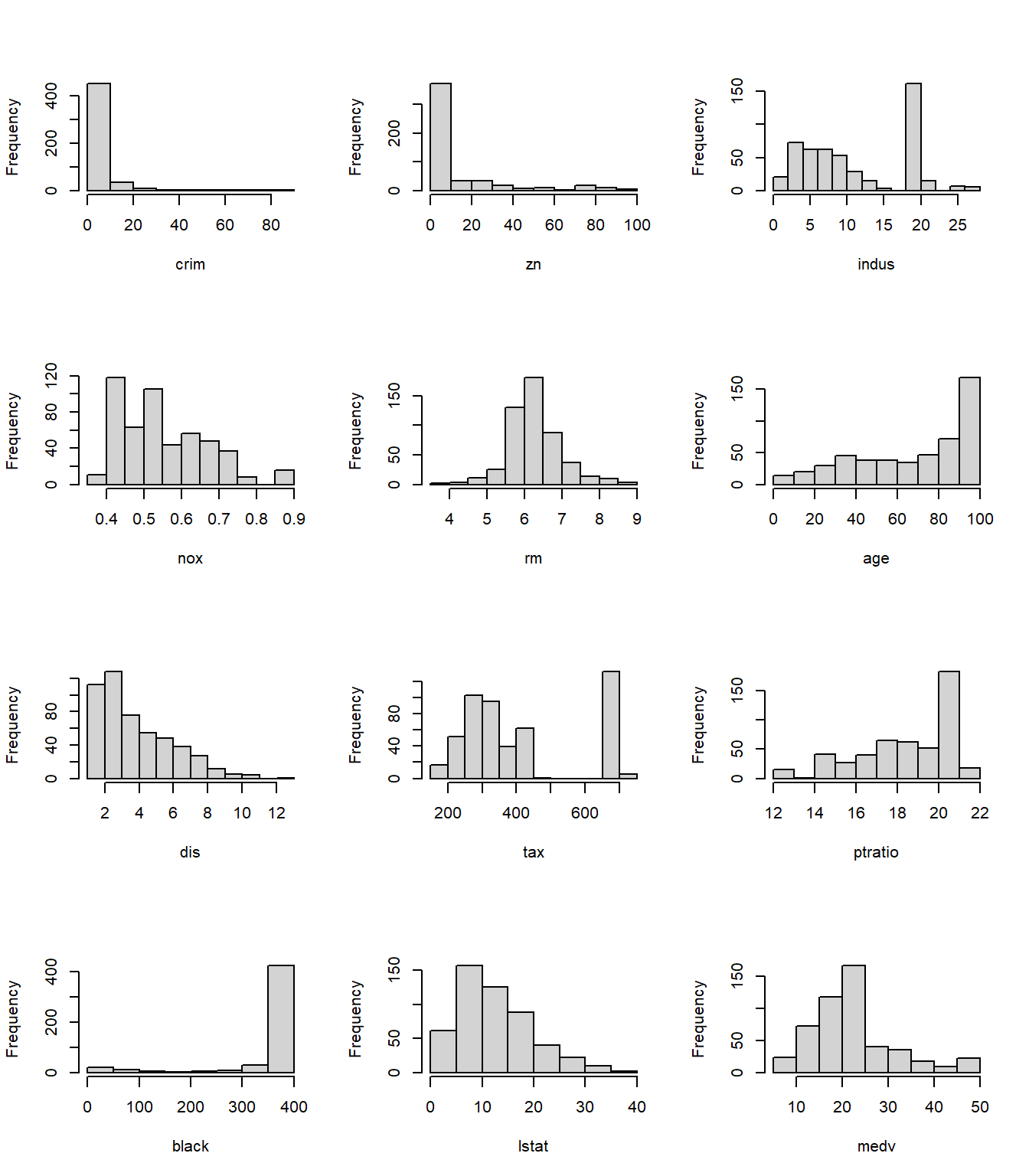
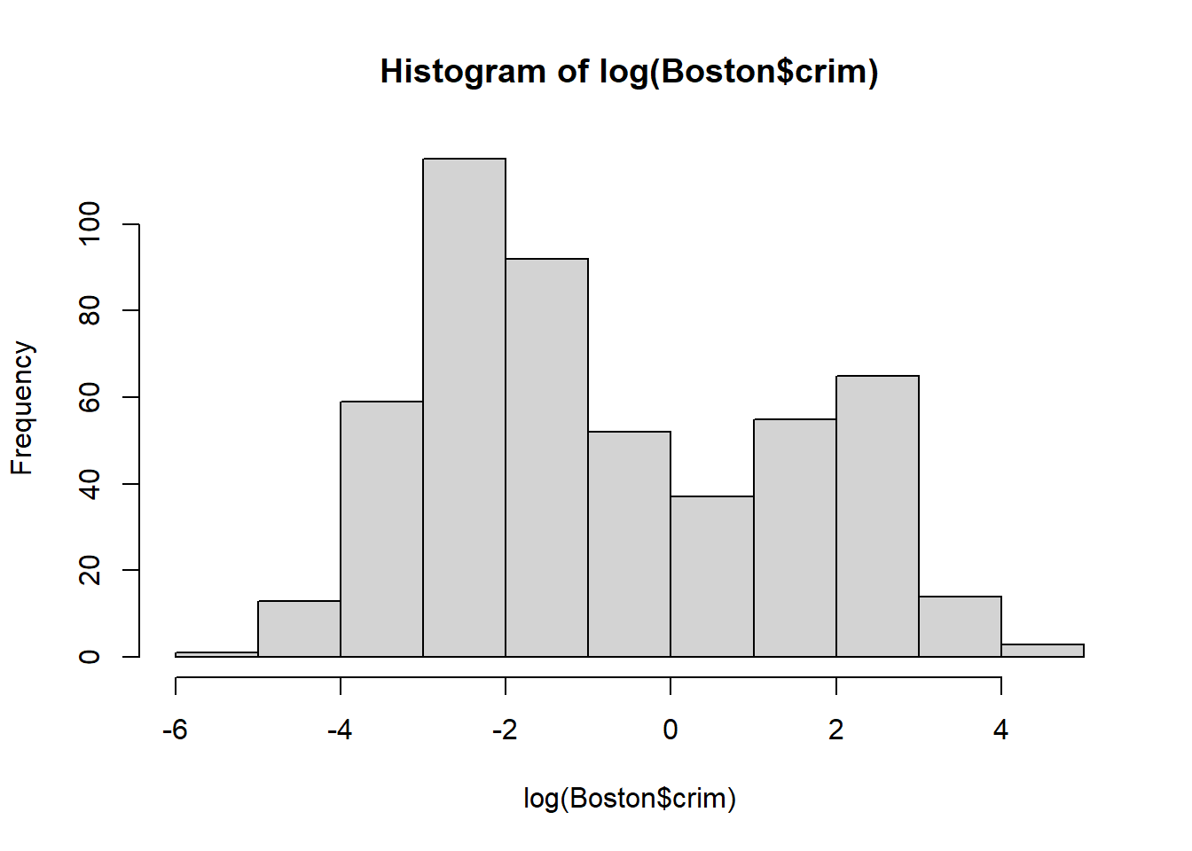
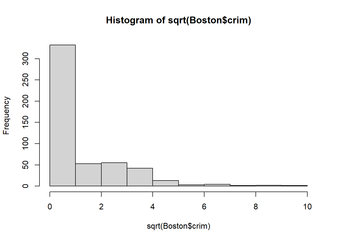
  • crim, zn, dis, black, and tax show strong skewness or long tails in the summary table, with crim especially right-skewed. This suggests that some nonlinear transformations may be useful.
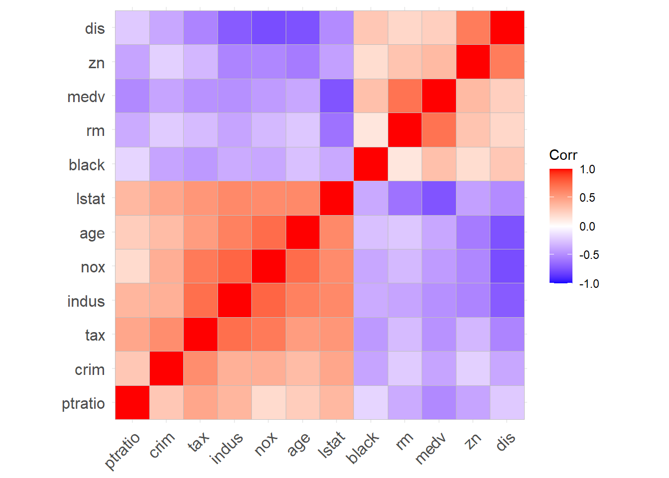
  • The correlation matrix confirms that medv is most strongly negatively correlated with lstat and positively correlated with rm, which matches what we see in the pair plots.
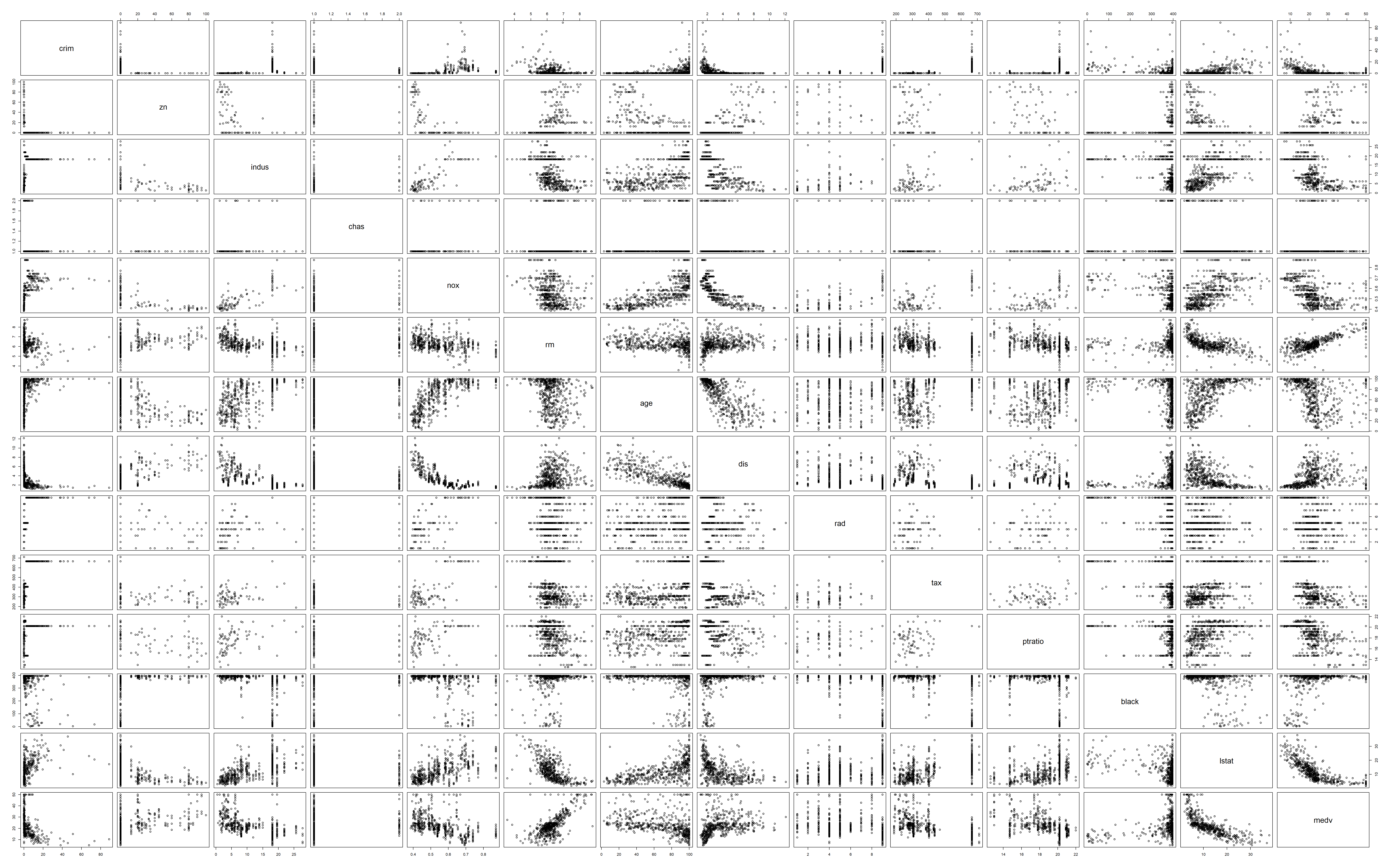
  • The pair plots show some curved pattern between medv and some variables like crim, rm and lstat. This is a strong sign that some nonlinear transformations will be needed.
  • nox, indus, age and dis are highly correlated, positive or negative. These variables all describe urban intensity or location-related structure, so multicollinearity is a concern.
  • We see no obvious extreme outliers based on the pair plots. However we still need to run diagnostics.

14.2 Step 2: Start with All Predictors — Full Model

We begin with the full additive regression model.

fit_full <- lm(medv ~ ., data = Boston)
summary(fit_full)

Call:
lm(formula = medv ~ ., data = Boston)

Residuals:
     Min       1Q   Median       3Q      Max 
-15.1020  -2.7355  -0.4565   1.6821  25.9450 

Coefficients:
              Estimate Std. Error t value Pr(>|t|)    
(Intercept)  35.259615   5.433641   6.489 2.14e-10 ***
crim         -0.108821   0.032685  -3.329 0.000937 ***
zn            0.054896   0.014149   3.880 0.000119 ***
indus         0.023760   0.063648   0.373 0.709081    
chas1         2.524163   0.863181   2.924 0.003614 ** 
nox         -17.573132   3.896362  -4.510 8.13e-06 ***
rm            3.665491   0.421196   8.703  < 2e-16 ***
age           0.000461   0.013227   0.035 0.972210    
dis          -1.554546   0.201909  -7.699 7.75e-14 ***
rad2          1.488905   1.477509   1.008 0.314095    
rad3          4.681254   1.335295   3.506 0.000498 ***
rad4          2.576234   1.187369   2.170 0.030514 *  
rad5          2.918493   1.207610   2.417 0.016028 *  
rad6          1.185839   1.464013   0.810 0.418342    
rad7          4.878992   1.571198   3.105 0.002012 ** 
rad8          4.839836   1.491657   3.245 0.001257 ** 
rad24         7.461674   1.788679   4.172 3.58e-05 ***
tax          -0.008748   0.003895  -2.246 0.025144 *  
ptratio      -0.972419   0.144478  -6.731 4.78e-11 ***
black         0.009394   0.002661   3.531 0.000454 ***
lstat        -0.529226   0.050640 -10.451  < 2e-16 ***
---
Signif. codes:  0 '***' 0.001 '**' 0.01 '*' 0.05 '.' 0.1 ' ' 1

Residual standard error: 4.694 on 485 degrees of freedom
Multiple R-squared:  0.7499,    Adjusted R-squared:  0.7396 
F-statistic:  72.7 on 20 and 485 DF,  p-value: < 2.2e-16

This model provides a baseline for comparison.

par(mfrow = c(2, 2))
plot(fit_full)
par(mfrow = c(1, 1))

Here are some important info we get.

  • \(R_{adj}^2\approx0.7395525\) and \(R^2\approx0.7498672\).
  • The overall F-test has a very small p-value, indicating that at least one predictor is associated with the response variable.
  • indus, age and some of the rad levels are not signicant.

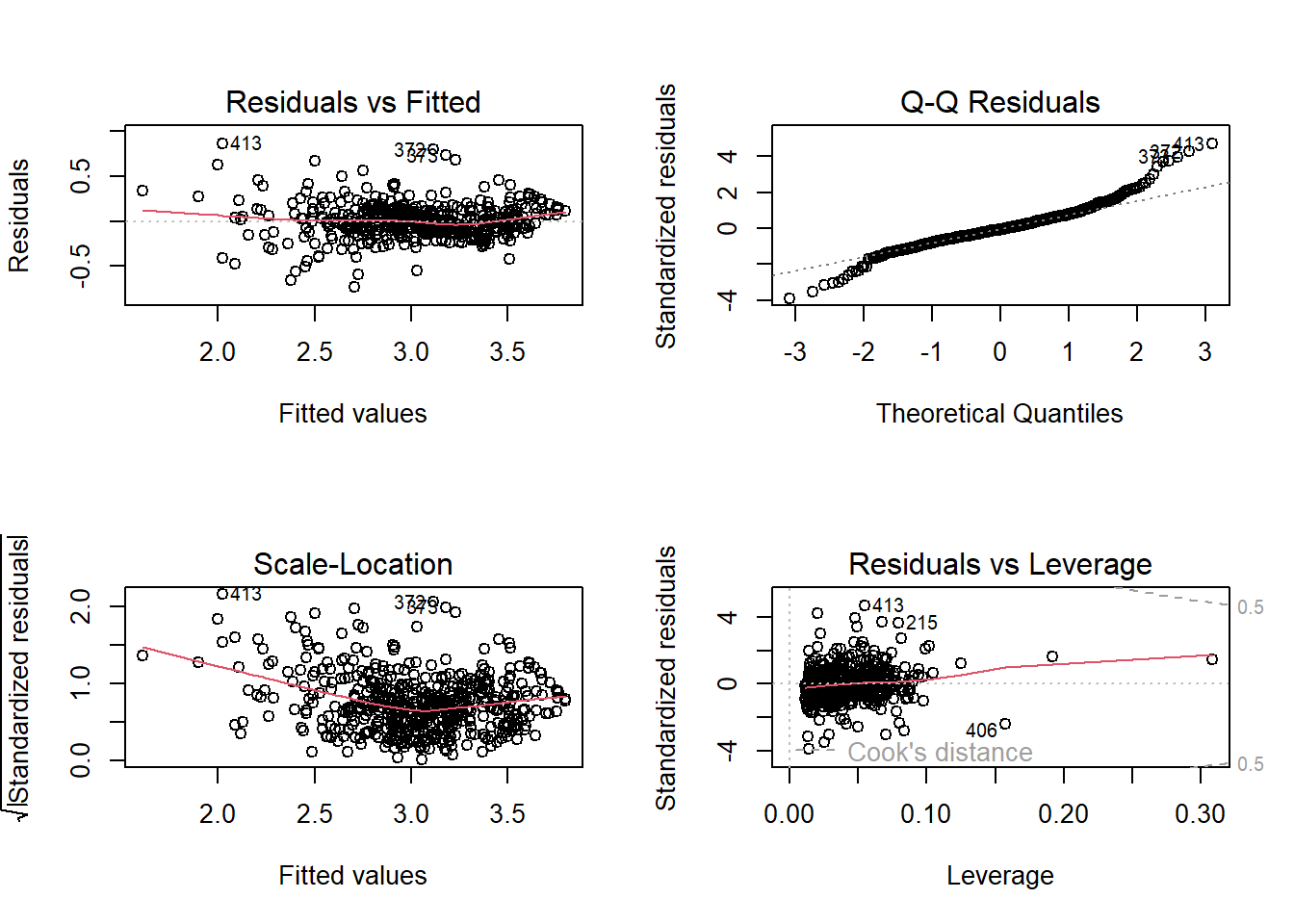
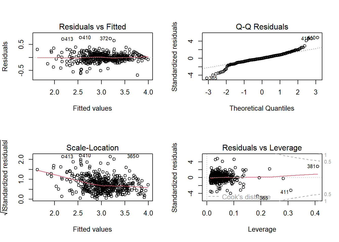
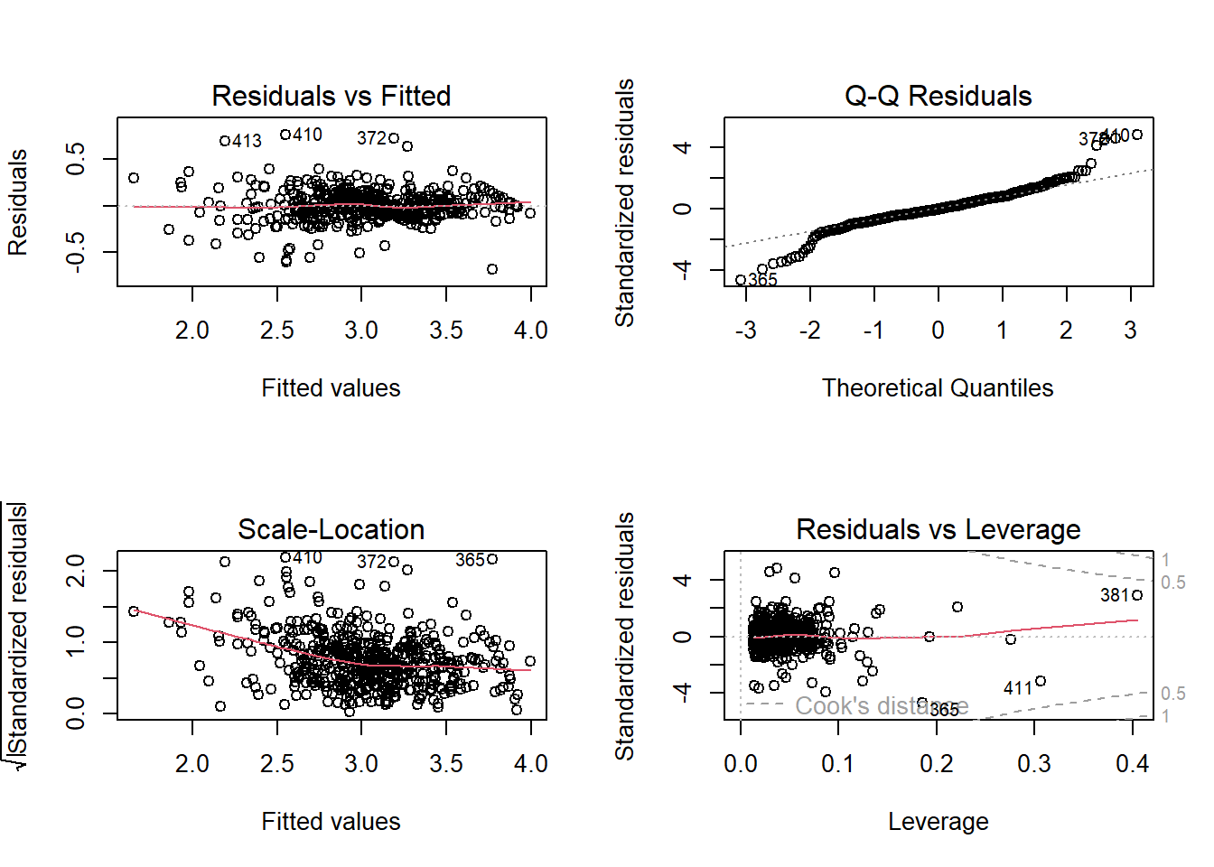
Then immediately do residual diagnostics on this full model:

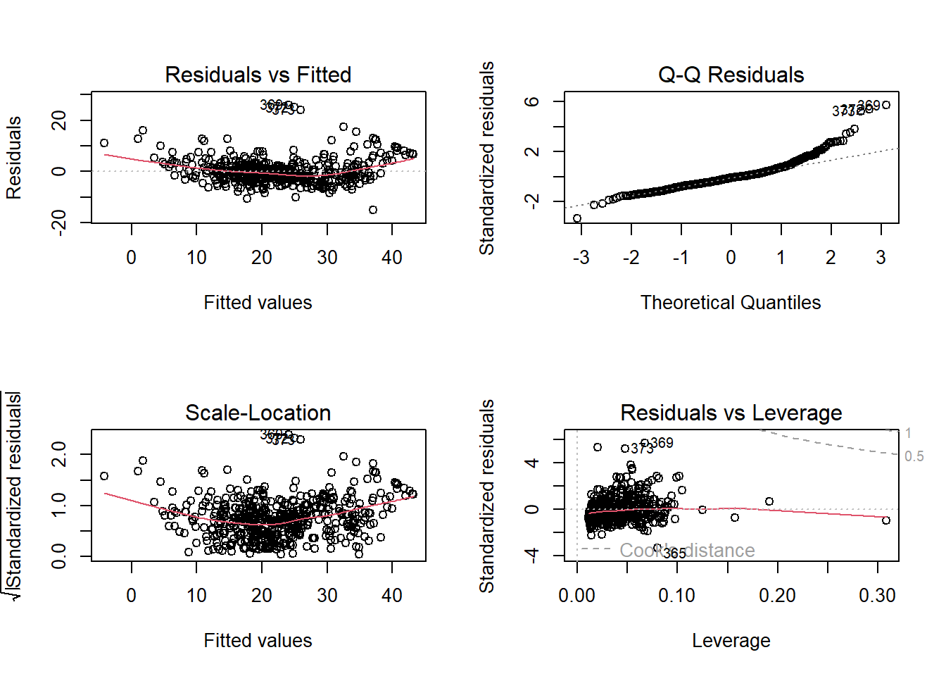
  1. From the residual plot, the red line is not flat, with a slight U-shape. In addition, residual variance increases slightly as fitted values increase.
  2. From the Q-Q plot, points follow the line in the middle, but right tail bends upward, and several points deviate strongly.
  3. From the scale-location plot, the red trend line has a slight U-shape, and the residual spread grows as fitted values increase.
  4. From the residuals vs leverage plot, most points have low leverage with one is around 0.30, and no points have large Cook’s distance.

These suggest the following observations:

  1. There are possible nonlinearity among variables.
  2. There is a possible heteroscedasticity.
  3. Residuals are not perfectly normal especially in the right tail.
  4. There are no extremely influential observations.

Based on all the observations (from this section and the previous section), we would like to start from applying some nonlinear transformations to build the model.

14.3 Step 3: Consider Transformations

14.3.1 Check if log(medv) improves things

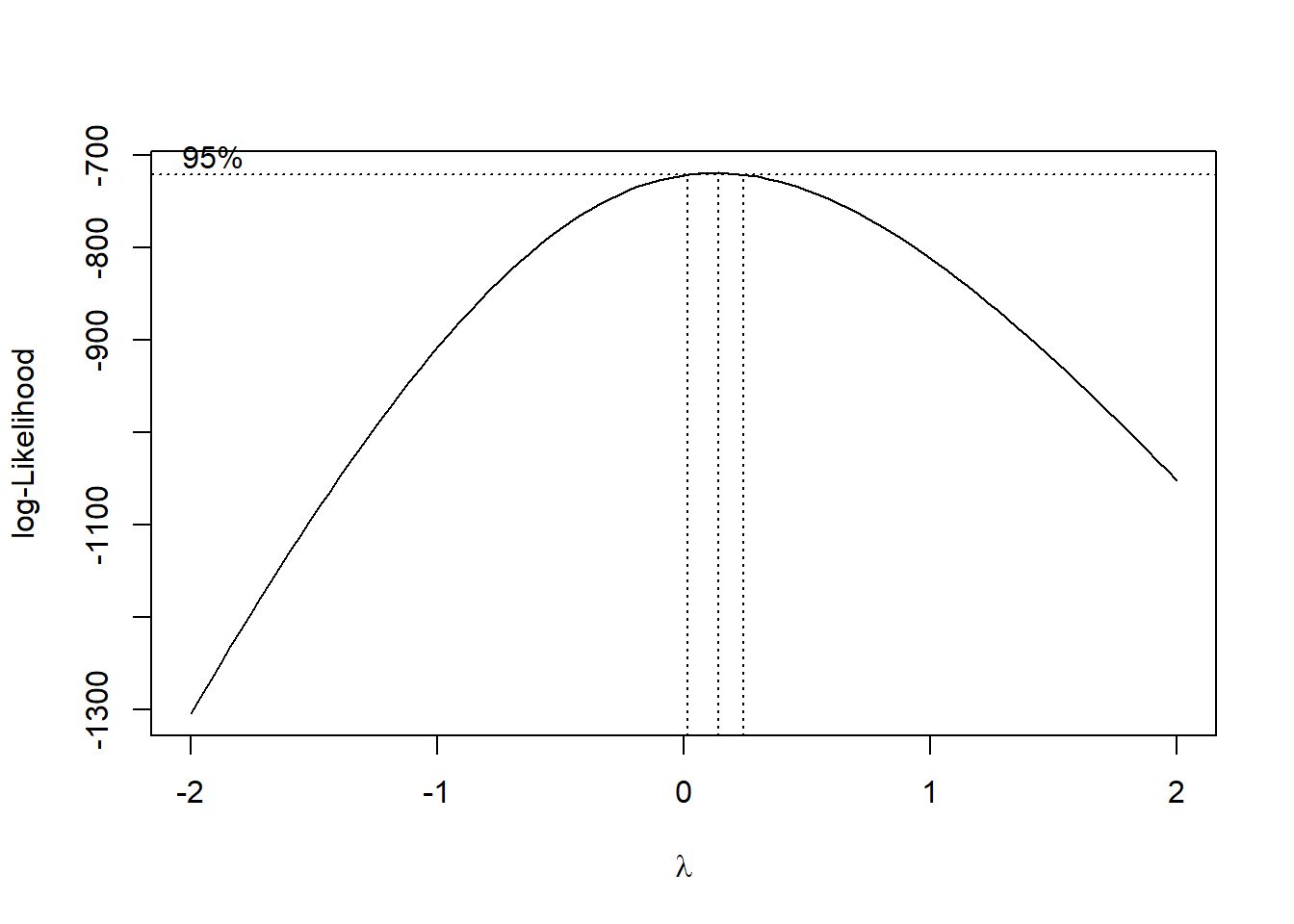
We begin by examining the response variable (because of the curvy residual plot and the slightly heteroscedasticity). To determine an appropriate transformation, we apply the Box–Cox procedure to search for a suitable power transformation of medv:

boxcox(fit_full)

The peak of the profile log-likelihood appears to occur around \(\lambda\approx0.1\). The \(95\%\) confidence interval for \(\lambda\) is slightly above \(0\), so \(0\) lies just outside the interval. This suggests that the optimal transformation is approximately \(y^{0.1}\). However, because \(0.1\) is very close to \(0\), the log transformation \(\log(y)\) is often used in practice. The log transformation is simpler, widely used, and produces a model fit very similar to the optimal Box–Cox transformation.

We therefore refit the model using log(medv) as the response.

fit_log <- lm(log(medv) ~ ., data = Boston)
summary(fit_log)

Call:
lm(formula = log(medv) ~ ., data = Boston)

Residuals:
     Min       1Q   Median       3Q      Max 
-0.73163 -0.10074 -0.01271  0.09153  0.86209 

Coefficients:
              Estimate Std. Error t value Pr(>|t|)    
(Intercept)  4.0078476  0.2188374  18.314  < 2e-16 ***
crim        -0.0102270  0.0013164  -7.769 4.75e-14 ***
zn           0.0015096  0.0005698   2.649 0.008333 ** 
indus        0.0027748  0.0025634   1.082 0.279575    
chas1        0.1002734  0.0347642   2.884 0.004096 ** 
nox         -0.7728738  0.1569242  -4.925 1.16e-06 ***
rm           0.0868708  0.0169635   5.121 4.39e-07 ***
age          0.0001981  0.0005327   0.372 0.710086    
dis         -0.0511276  0.0081318  -6.287 7.21e-10 ***
rad2         0.0833711  0.0595060   1.401 0.161838    
rad3         0.1766617  0.0537784   3.285 0.001094 ** 
rad4         0.1002350  0.0478207   2.096 0.036595 *  
rad5         0.1344828  0.0486359   2.765 0.005908 ** 
rad6         0.0961606  0.0589625   1.631 0.103565    
rad7         0.2075191  0.0632793   3.279 0.001115 ** 
rad8         0.1939560  0.0600758   3.229 0.001329 ** 
rad24        0.3504602  0.0720382   4.865 1.55e-06 ***
tax         -0.0005052  0.0001569  -3.221 0.001365 ** 
ptratio     -0.0370069  0.0058188  -6.360 4.67e-10 ***
black        0.0004148  0.0001072   3.871 0.000123 ***
lstat       -0.0291645  0.0020395 -14.300  < 2e-16 ***
---
Signif. codes:  0 '***' 0.001 '**' 0.01 '*' 0.05 '.' 0.1 ' ' 1

Residual standard error: 0.189 on 485 degrees of freedom
Multiple R-squared:  0.7946,    Adjusted R-squared:  0.7861 
F-statistic: 93.81 on 20 and 485 DF,  p-value: < 2.2e-16
par(mfrow = c(2, 2))
plot(fit_log)
par(mfrow = c(1, 1))

With log(medv) as the response:

  • Coefficients are interpreted as the approximate percentage change in the median of medv associated with a one-unit increase in the predictor, holding other variables constant.
  • \(R_{adj}^2\) and \(R^2\) increase slightly, indicating a small improvement in model fit.
  • However, the diagnostic plots show that the main issues (nonlinearity, heteroscedasticity, and non-normal residuals) are not substantially improved.

Therefore, transforming the response alone is not sufficient, and we need to consider additional model modifications, such as transformations of predictors, interaction terms, or nonlinear terms.

NoteInterpretation of \(\log(y)\)

Assume \[ \log(y)=\beta_0+\sum_{i=1}^k{\beta_i x_i}+\varepsilon=\beta_0+\mathbf{\beta_1x}+\varepsilon \] Then \[ y=\me^{\beta_0}\me^{\mathbf{\beta_1x}}\me^{\varepsilon}=\me^{\beta_0+\varepsilon}\me^{\mathbf{\beta_1x}}. \] Therefore if \(\mathbf{\Delta x}=[\Delta x_1,\Delta x_2,\ldots,\Delta x_k]\) are all small, \[ \begin{split} \Delta y/y&=\qty(\me^{\beta_0+\varepsilon}\me^{\mathbf{\beta_1(x+\Delta x)}}-\me^{\beta_0+\varepsilon}\me^{\mathbf{\beta_1x}})/\me^{\beta_0+\varepsilon}\me^{\mathbf{\beta_1x}}=\qty(\me^{\mathbf{\beta_1(x+\Delta x)}}-\me^{\mathbf{\beta_1x}})/\me^{\mathbf{\beta_1x}}=\me^{\mathbf{\beta_1\Delta x}}-1\\ &\approx 1+\mathbf{\beta_1 \Delta x}-1=\mathbf{\beta_1 \Delta x}=\sum_{i=1}^k{\beta_i \Delta x_i}. \end{split} \] Then the interpretation should be:

A one-unit increase in \(x_i\) is associated with an approximate \(100 \cdot \beta_i \%\) change in the median of \(y\), holding all other predictors constant.

CautionThe “Mean vs. Median” Trap

When we assume the errors \(\varepsilon \sim N(0, \sigma^2)\) are symmetric, our OLS model estimates the conditional mean of \(\log(y)\). However, due to Jensen’s Inequality, \(e^{\operatorname{E}[\log(y)]}\) does not equal \(\operatorname{E}[y]\). Instead:

  • \(\me^{\hat{y}}\) provides an estimate of the Median of \(y\).
  • The Mean of \(y\) is actually shifted by a correction factor: \(\operatorname{E}[y] = \text{Median}(y) \cdot \me^{\sigma^2/2}\).

If you do not wish to apply the correction factor, you should strictly interpret your results as the percentage change in the median of \(y\) rather than the mean, just like what we did in the above note block.

14.3.2 Partial residual plots

Then we look at the partial residual plots.

First show the partial residual plots.

par(mfrow = c(4, 3))
crPlots(fit_log)
par(mfrow = c(1, 1))

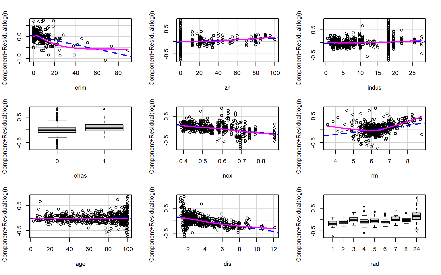
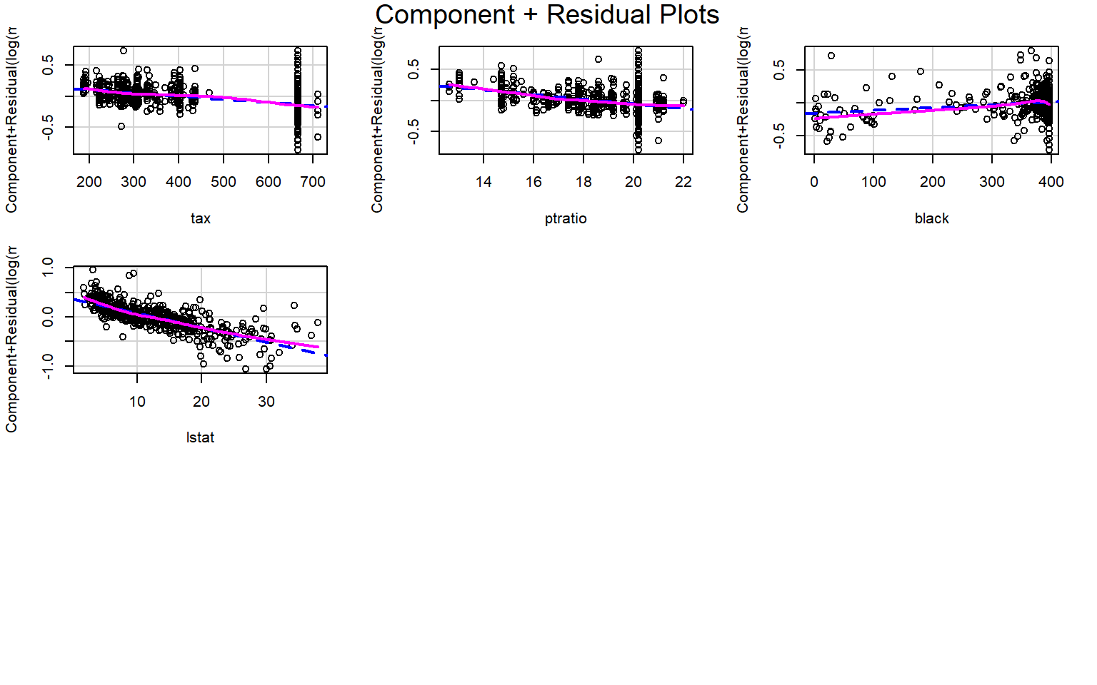
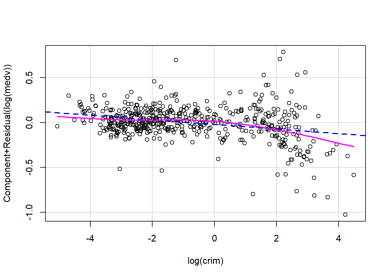
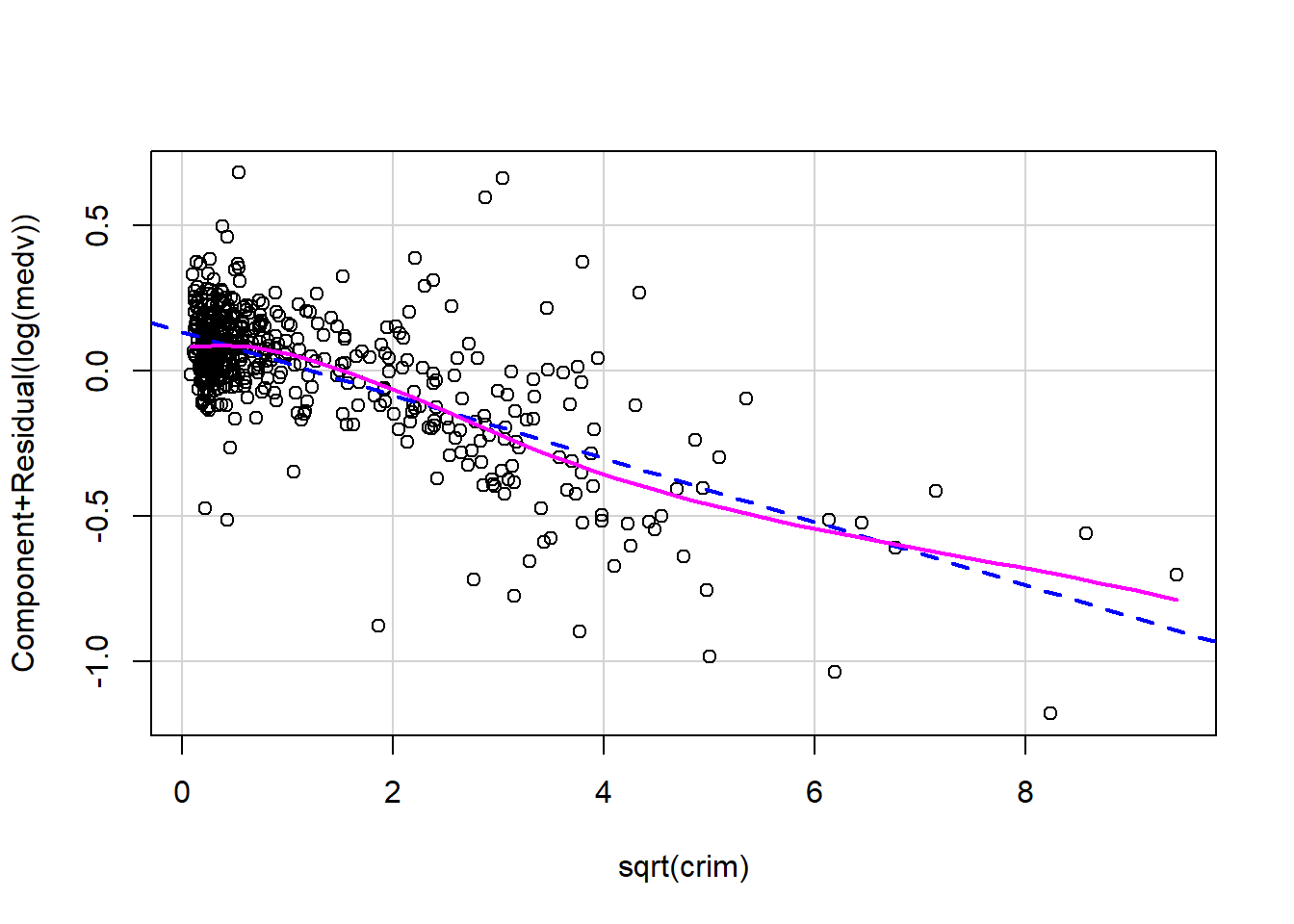
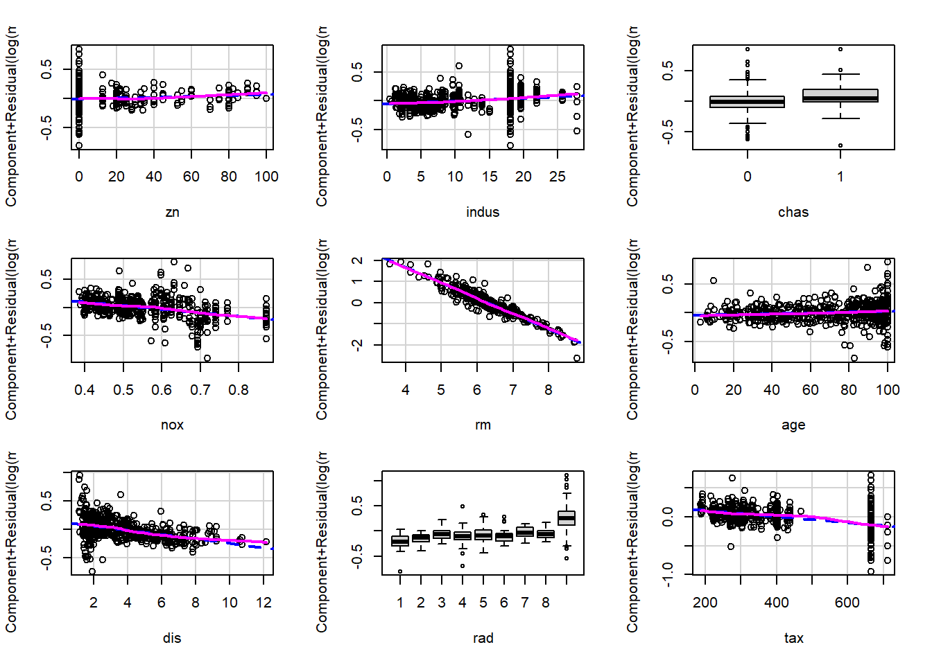
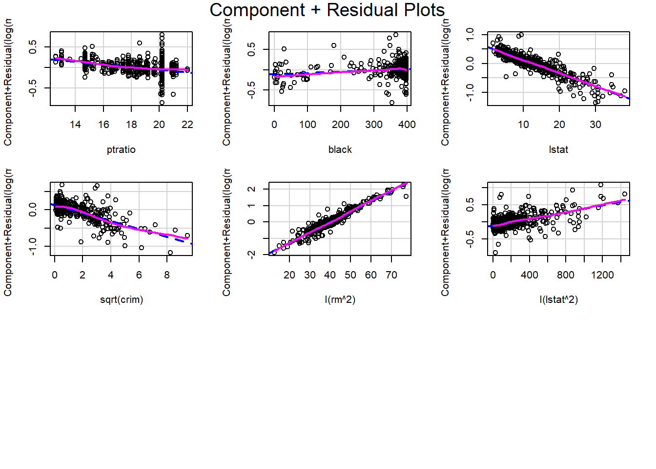
Based on the partial residual plots, it appears that crim, rm, and lstat exhibit some curvature. Therefore, we consider applying transformations to these variables.

From the earlier EDA, we observed that crim is strongly right-skewed. A common way to address this is to apply a transformation such as log(crim) or sqrt(crim), both of which reduce right skewness by compressing larger values. In either case, the original variable crim must be removed from the model and replaced by its transformed version.

To determine which transformation is more appropriate, we compare their model performance and examine the corresponding partial residual plots.

We first consider the log(crim) transformation.

fit_logcrim <- lm(
    log(medv) ~ . - crim + log(crim) + I(rm^2) + I(lstat^2),
    data = Boston
)
summary(fit_logcrim)

Call:
lm(formula = log(medv) ~ . - crim + log(crim) + I(rm^2) + I(lstat^2), 
    data = Boston)

Residuals:
     Min       1Q   Median       3Q      Max 
-0.89730 -0.09521 -0.00077  0.09639  0.86267 

Coefficients:
              Estimate Std. Error t value Pr(>|t|)    
(Intercept)  6.2627356  0.4503587  13.906  < 2e-16 ***
zn           0.0003599  0.0005961   0.604 0.546268    
indus        0.0056910  0.0025803   2.206 0.027886 *  
chas1        0.1053075  0.0348290   3.024 0.002631 ** 
nox         -0.5908938  0.1637875  -3.608 0.000341 ***
rm          -0.7211240  0.1349247  -5.345 1.40e-07 ***
age          0.0005285  0.0005590   0.945 0.344930    
dis         -0.0319884  0.0082824  -3.862 0.000128 ***
rad2         0.0909897  0.0596367   1.526 0.127731    
rad3         0.1879332  0.0544635   3.451 0.000608 ***
rad4         0.1313052  0.0503649   2.607 0.009414 ** 
rad5         0.1612607  0.0499684   3.227 0.001335 ** 
rad6         0.1555609  0.0601487   2.586 0.009994 ** 
rad7         0.2137491  0.0658468   3.246 0.001251 ** 
rad8         0.1809895  0.0639362   2.831 0.004837 ** 
rad24        0.3188068  0.0837593   3.806 0.000159 ***
tax         -0.0005060  0.0001571  -3.220 0.001367 ** 
ptratio     -0.0306837  0.0059746  -5.136 4.08e-07 ***
black        0.0004187  0.0001083   3.864 0.000127 ***
lstat       -0.0421794  0.0061665  -6.840 2.40e-11 ***
log(crim)   -0.0258154  0.0117888  -2.190 0.029014 *  
I(rm^2)      0.0631674  0.0105952   5.962 4.82e-09 ***
I(lstat^2)   0.0002960  0.0001622   1.825 0.068613 .  
---
Signif. codes:  0 '***' 0.001 '**' 0.01 '*' 0.05 '.' 0.1 ' ' 1

Residual standard error: 0.1894 on 483 degrees of freedom
Multiple R-squared:  0.7947,    Adjusted R-squared:  0.7854 
F-statistic:    85 on 22 and 483 DF,  p-value: < 2.2e-16
crPlot(fit_logcrim, "log(crim)")

Then we consider the sqrt(crim) transformation.

fit_sqrtcrim <- lm(
    log(medv) ~ . - crim + sqrt(crim) + I(rm^2) + I(lstat^2),
    data = Boston
)
summary(fit_sqrtcrim)

Call:
lm(formula = log(medv) ~ . - crim + sqrt(crim) + I(rm^2) + I(lstat^2), 
    data = Boston)

Residuals:
     Min       1Q   Median       3Q      Max 
-0.80769 -0.09297 -0.00499  0.09335  0.85847 

Coefficients:
              Estimate Std. Error t value Pr(>|t|)    
(Intercept)  6.5867162  0.4193760  15.706  < 2e-16 ***
zn           0.0007401  0.0005373   1.377 0.169026    
indus        0.0048775  0.0023898   2.041 0.041796 *  
chas1        0.0883226  0.0323541   2.730 0.006567 ** 
nox         -0.6367620  0.1460046  -4.361 1.58e-05 ***
rm          -0.7330235  0.1247380  -5.877 7.82e-09 ***
age          0.0007048  0.0005148   1.369 0.171567    
dis         -0.0380612  0.0077148  -4.934 1.11e-06 ***
rad2         0.0696192  0.0553303   1.258 0.208910    
rad3         0.1744046  0.0499968   3.488 0.000531 ***
rad4         0.1171443  0.0445411   2.630 0.008810 ** 
rad5         0.1497328  0.0452229   3.311 0.000999 ***
rad6         0.1336138  0.0551389   2.423 0.015750 *  
rad7         0.2051604  0.0590059   3.477 0.000553 ***
rad8         0.1683402  0.0563126   2.989 0.002938 ** 
rad24        0.4868403  0.0718538   6.775 3.62e-11 ***
tax         -0.0005255  0.0001458  -3.604 0.000346 ***
ptratio     -0.0326013  0.0054886  -5.940 5.46e-09 ***
black        0.0002955  0.0001007   2.933 0.003515 ** 
lstat       -0.0461610  0.0057383  -8.044 6.76e-15 ***
sqrt(crim)  -0.1086725  0.0118773  -9.150  < 2e-16 ***
I(rm^2)      0.0634084  0.0097960   6.473 2.37e-10 ***
I(lstat^2)   0.0004894  0.0001520   3.219 0.001372 ** 
---
Signif. codes:  0 '***' 0.001 '**' 0.01 '*' 0.05 '.' 0.1 ' ' 1

Residual standard error: 0.1757 on 483 degrees of freedom
Multiple R-squared:  0.8233,    Adjusted R-squared:  0.8153 
F-statistic: 102.3 on 22 and 483 DF,  p-value: < 2.2e-16
crPlot(fit_sqrtcrim, "sqrt(crim)")

hist(log(Boston$crim))
hist(sqrt(Boston$crim))

AIC(fit_logcrim, fit_sqrtcrim)
             df       AIC
fit_logcrim  24 -223.6377
fit_sqrtcrim 24 -299.5182

Based on the results above:

  • Both transformations substantially straighten the partial residual plot, indicating that the nonlinear pattern in crim is largely removed.
  • From the partial residual plots alone, it is difficult to determine which transformation is preferable.
  • From the perspective of the variable distribution, log(crim) spreads the data more evenly than sqrt(crim).
  • However, in terms of model performance, such as \(R^2_{adj}\) and AIC, the model using sqrt(crim) performs slightly better. In particular, the AIC is slightly smaller, indicating a better balance between goodness of fit and model complexity.

Taking all these considerations into account, we choose to use sqrt(crim) in the model. Under this transformation, the effect of crim on log(medv) becomes nonlinear: the marginal impact of crime decreases as crim increases, meaning that the slope becomes smaller for larger values of crim.

We then examine the full set of partial residual plots again to check for any remaining unusual patterns. No additional strong nonlinear effects are observed.

par(mfrow = c(4, 3))
crPlots(fit_sqrtcrim)
par(mfrow = c(1, 1))

Finally we use nested F-test to confirm the addition.

fit_sc <- lm(log(medv) ~ . - crim + sqrt(crim), data=Boston)
anova(fit_sc, fit_sqrtcrim)
Analysis of Variance Table

Model 1: log(medv) ~ (crim + zn + indus + chas + nox + rm + age + dis + 
    rad + tax + ptratio + black + lstat) - crim + sqrt(crim)
Model 2: log(medv) ~ (crim + zn + indus + chas + nox + rm + age + dis + 
    rad + tax + ptratio + black + lstat) - crim + sqrt(crim) + 
    I(rm^2) + I(lstat^2)
  Res.Df    RSS Df Sum of Sq      F    Pr(>F)    
1    485 17.551                                  
2    483 14.908  2    2.6436 42.826 < 2.2e-16 ***
---
Signif. codes:  0 '***' 0.001 '**' 0.01 '*' 0.05 '.' 0.1 ' ' 1

This shows that rm^2 and lstat^2 are significant to be added. For crim, since we replace it with sqrt(crim) instead of adding a term, we cannot directly use the nested ANOVA since these are not nested models. We then use AIC to test which model is better.

fit_sc2 <- lm(log(medv) ~ . + I(rm^2) + I(lstat^2), data = Boston)
AIC(fit_sc2, fit_sqrtcrim)
             df       AIC
fit_sc2      24 -299.0543
fit_sqrtcrim 24 -299.5182

fit_sqrtcrim has a slightly lower AIC. Therefore we would go with fit_sqrtcrim as our transformed variable model.

14.3.3 Interaction terms

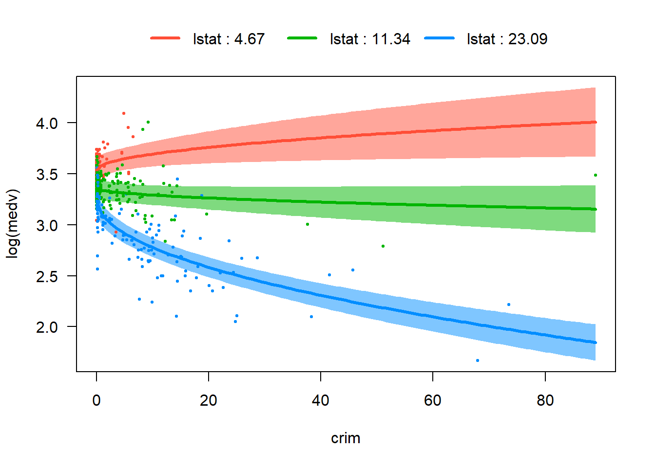
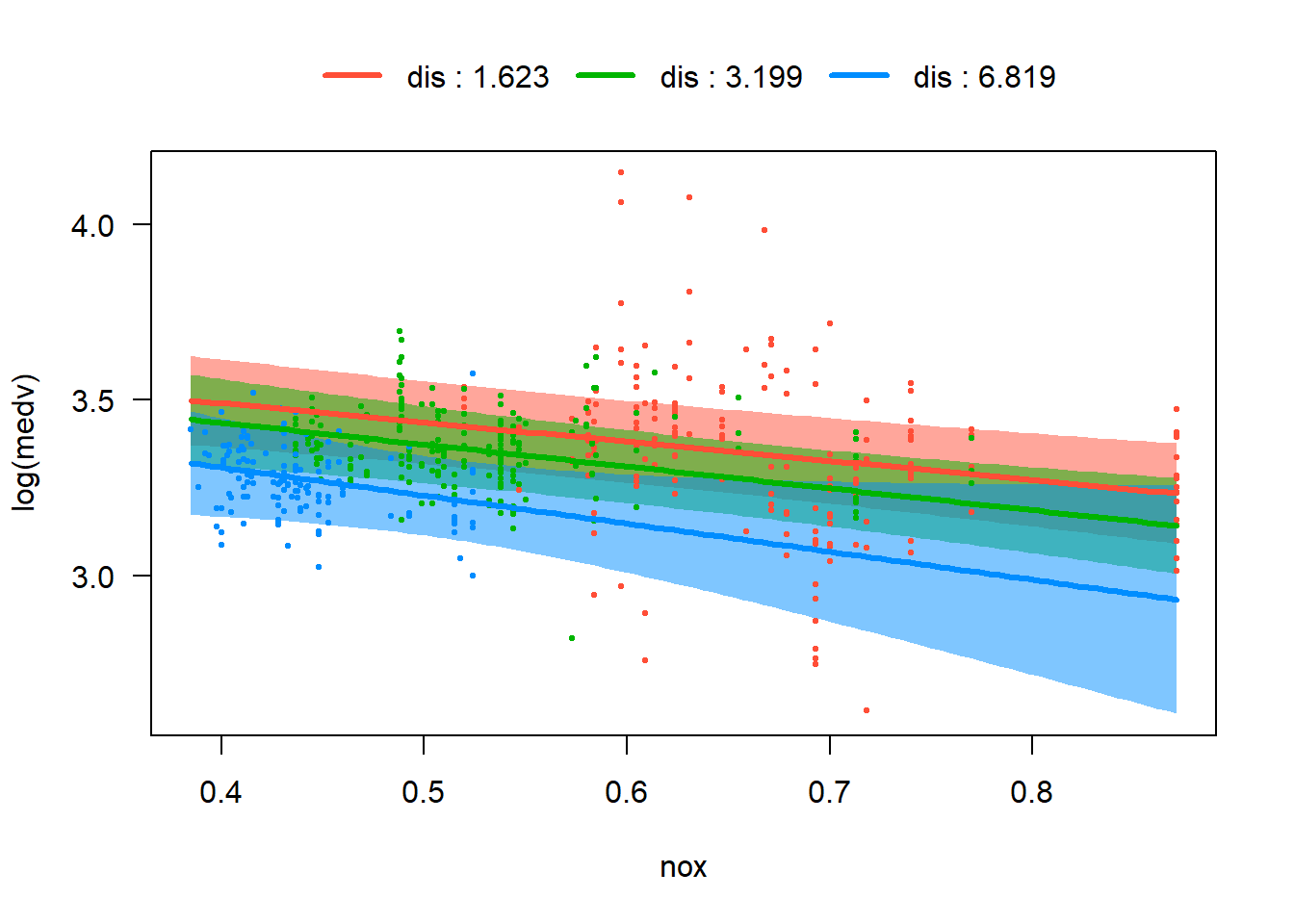
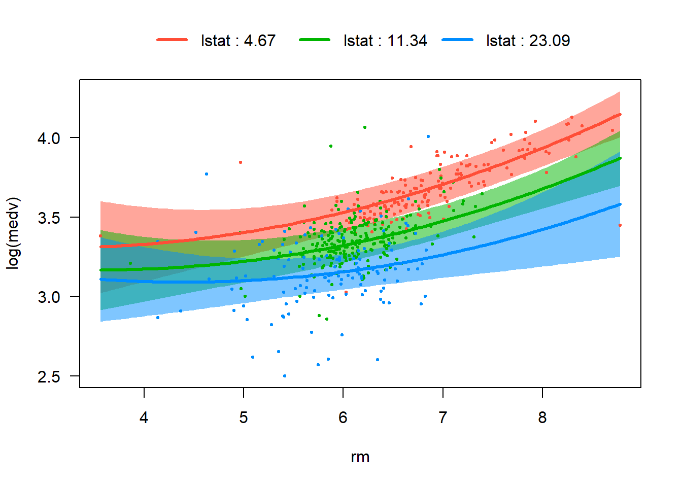
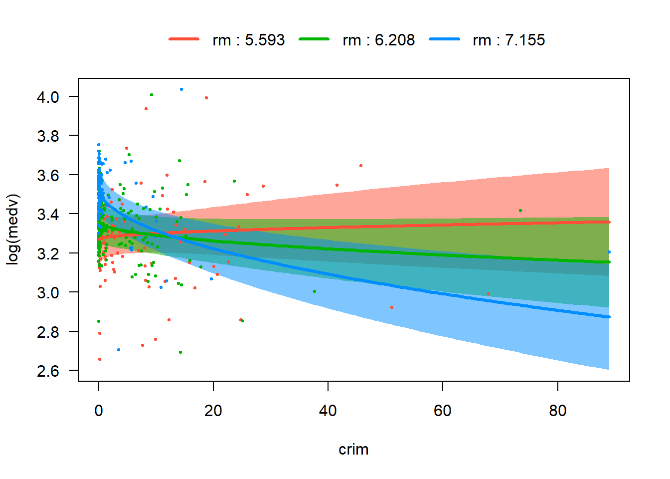
In the Boston housing dataset, some pairs of predictors naturally suggest possible interaction terms. For instance, crim and lstat both reflect neighborhood socioeconomic conditions, so the impact of crime on housing price may depend on the socioeconomic status of the neighborhood. The variables nox and dis may also interact, since pollution and distance to employment centers jointly describe environmental and location quality. In addition, rm and lstat could interact because the value added by larger houses may differ across neighborhoods with different income levels. Exploring these interaction terms helps determine whether the relationship between predictors and the response changes across different conditions.

Possible interaction terms in the Boston dataset include:

  • crim × lstat: crime and socioeconomic status both describe neighborhood disadvantage.
  • nox × dis: pollution and distance jointly characterize environmental and location quality.
  • rm × lstat: the value of larger houses may depend on neighborhood socioeconomic status.
  • rm × crim: the price premium of larger houses may differ in high-crime areas.

We first use visreg to quickly screen these ideas.

library(visreg)
fit_ints <- lm(
    log(medv) ~ . - crim + sqrt(crim) + I(rm^2) + I(lstat^2) + sqrt(crim)*lstat + nox*dis + rm*lstat + sqrt(crim)*rm,
    data = Boston
)
visreg(fit_ints, "crim", by = "lstat", overlay = TRUE)

visreg(fit_ints, "nox", by = "dis", overlay = TRUE)

visreg(fit_ints, "rm", by = "lstat", overlay = TRUE)

visreg(fit_ints, "crim", by = "rm", overlay = TRUE)

From these four plots, we are able to visualize differences in slopes across levels of the interacting variable. However nox bydis and rm by lstat are weaker, and their p-values are relative big. Therefore we would only keep lstat:sqrt(crim) and rm:sqrt(crim) in our tentative model and proceed to the next test phase.

fit_int <- lm(
    log(medv) ~ . - crim + sqrt(crim) + I(rm^2) + I(lstat^2) + sqrt(crim)*lstat + sqrt(crim)*rm,
    data = Boston
)

summary(fit_int)

Call:
lm(formula = log(medv) ~ . - crim + sqrt(crim) + I(rm^2) + I(lstat^2) + 
    sqrt(crim) * lstat + sqrt(crim) * rm, data = Boston)

Residuals:
     Min       1Q   Median       3Q      Max 
-0.68312 -0.07315 -0.00797  0.08404  0.76102 

Coefficients:
                   Estimate Std. Error t value Pr(>|t|)    
(Intercept)       4.497e+00  5.346e-01   8.412 4.63e-16 ***
zn                6.830e-04  4.990e-04   1.369 0.171751    
indus             1.444e-03  2.252e-03   0.641 0.521825    
chas1             6.892e-02  2.995e-02   2.301 0.021799 *  
nox              -5.663e-01  1.355e-01  -4.180 3.46e-05 ***
rm               -2.340e-01  1.432e-01  -1.634 0.102888    
age              -3.385e-04  4.885e-04  -0.693 0.488688    
dis              -3.716e-02  7.157e-03  -5.192 3.08e-07 ***
rad2              5.256e-02  5.104e-02   1.030 0.303563    
rad3              1.453e-01  4.622e-02   3.143 0.001774 ** 
rad4              8.935e-02  4.122e-02   2.168 0.030662 *  
rad5              1.322e-01  4.176e-02   3.166 0.001645 ** 
rad6              1.233e-01  5.086e-02   2.424 0.015727 *  
rad7              1.625e-01  5.458e-02   2.978 0.003049 ** 
rad8              1.330e-01  5.204e-02   2.555 0.010916 *  
rad24             4.014e-01  6.686e-02   6.003 3.82e-09 ***
tax              -5.485e-04  1.345e-04  -4.077 5.34e-05 ***
ptratio          -2.723e-02  5.094e-03  -5.345 1.40e-07 ***
black             3.368e-04  9.297e-05   3.623 0.000322 ***
lstat            -4.494e-02  5.666e-03  -7.932 1.52e-14 ***
sqrt(crim)        4.706e-01  8.301e-02   5.670 2.47e-08 ***
I(rm^2)           3.285e-02  1.035e-02   3.173 0.001605 ** 
I(lstat^2)        1.092e-03  1.653e-04   6.604 1.06e-10 ***
lstat:sqrt(crim) -1.098e-02  1.175e-03  -9.342  < 2e-16 ***
rm:sqrt(crim)    -5.876e-02  1.122e-02  -5.238 2.43e-07 ***
---
Signif. codes:  0 '***' 0.001 '**' 0.01 '*' 0.05 '.' 0.1 ' ' 1

Residual standard error: 0.1619 on 481 degrees of freedom
Multiple R-squared:  0.8505,    Adjusted R-squared:  0.8431 
F-statistic:   114 on 24 and 481 DF,  p-value: < 2.2e-16
par(mfrow = c(2, 2))
plot(fit_int)
par(mfrow = c(1, 1))

All plots look good. Finally We use a nested ANOVA to confirm the addition.

anova(fit_sqrtcrim, fit_int)
Analysis of Variance Table

Model 1: log(medv) ~ (crim + zn + indus + chas + nox + rm + age + dis + 
    rad + tax + ptratio + black + lstat) - crim + sqrt(crim) + 
    I(rm^2) + I(lstat^2)
Model 2: log(medv) ~ (crim + zn + indus + chas + nox + rm + age + dis + 
    rad + tax + ptratio + black + lstat) - crim + sqrt(crim) + 
    I(rm^2) + I(lstat^2) + sqrt(crim) * lstat + sqrt(crim) * 
    rm
  Res.Df    RSS Df Sum of Sq      F    Pr(>F)    
1    483 14.908                                  
2    481 12.612  2    2.2955 43.774 < 2.2e-16 ***
---
Signif. codes:  0 '***' 0.001 '**' 0.01 '*' 0.05 '.' 0.1 ' ' 1

Therefore we would like to use fit_int as our next step.

14.3.4 Variable selections

We apply best-of-subset to select variables since this model doesn’t contain too many variables.

library(leaps)
fits <- regsubsets(
    log(medv) ~ . - crim + sqrt(crim) + I(rm^2) + I(lstat^2) + sqrt(crim) * lstat + sqrt(crim) * rm,
    data = Boston,
    nvmax = ncol(model.matrix(log(medv) ~ . - crim + sqrt(crim) + I(rm^2) + I(lstat^2) + sqrt(crim) * lstat + sqrt(crim) * rm, Boston)) - 1
)
models_summary <- summary(fits)
best_cp <- which.min(models_summary$cp)
plot(models_summary$cp, xlab = "Number of varaiables", type = "l")
points(best_cp, models_summary$cp[best_cp], col = "red", cex = 2, pch = 20)

models_summary
Subset selection object
Call: regsubsets.formula(log(medv) ~ . - crim + sqrt(crim) + I(rm^2) + 
    I(lstat^2) + sqrt(crim) * lstat + sqrt(crim) * rm, data = Boston, 
    nvmax = ncol(model.matrix(log(medv) ~ . - crim + sqrt(crim) + 
        I(rm^2) + I(lstat^2) + sqrt(crim) * lstat + sqrt(crim) * 
        rm, Boston)) - 1)
24 Variables  (and intercept)
                 Forced in Forced out
zn                   FALSE      FALSE
indus                FALSE      FALSE
chas1                FALSE      FALSE
nox                  FALSE      FALSE
rm                   FALSE      FALSE
age                  FALSE      FALSE
dis                  FALSE      FALSE
rad2                 FALSE      FALSE
rad3                 FALSE      FALSE
rad4                 FALSE      FALSE
rad5                 FALSE      FALSE
rad6                 FALSE      FALSE
rad7                 FALSE      FALSE
rad8                 FALSE      FALSE
rad24                FALSE      FALSE
tax                  FALSE      FALSE
ptratio              FALSE      FALSE
black                FALSE      FALSE
lstat                FALSE      FALSE
sqrt(crim)           FALSE      FALSE
I(rm^2)              FALSE      FALSE
I(lstat^2)           FALSE      FALSE
lstat:sqrt(crim)     FALSE      FALSE
rm:sqrt(crim)        FALSE      FALSE
1 subsets of each size up to 24
Selection Algorithm: exhaustive
          zn  indus chas1 nox rm  age dis rad2 rad3 rad4 rad5 rad6 rad7 rad8
1  ( 1 )  " " " "   " "   " " " " " " " " " "  " "  " "  " "  " "  " "  " " 
2  ( 1 )  " " " "   " "   " " " " " " " " " "  " "  " "  " "  " "  " "  " " 
3  ( 1 )  " " " "   " "   " " " " " " " " " "  " "  " "  " "  " "  " "  " " 
4  ( 1 )  " " " "   " "   " " "*" " " " " " "  " "  " "  " "  " "  " "  " " 
5  ( 1 )  " " " "   " "   " " "*" " " " " " "  " "  " "  " "  " "  " "  " " 
6  ( 1 )  " " " "   " "   " " " " " " " " " "  " "  " "  " "  " "  " "  " " 
7  ( 1 )  " " " "   " "   " " " " " " " " " "  " "  " "  " "  " "  " "  " " 
8  ( 1 )  " " " "   " "   " " " " " " " " " "  " "  " "  " "  " "  " "  " " 
9  ( 1 )  " " " "   " "   "*" " " " " "*" " "  " "  " "  " "  " "  " "  " " 
10  ( 1 ) " " " "   " "   " " " " " " "*" " "  " "  " "  " "  " "  " "  " " 
11  ( 1 ) " " " "   " "   "*" " " " " "*" " "  " "  " "  " "  " "  " "  " " 
12  ( 1 ) " " " "   " "   "*" " " " " "*" " "  " "  " "  " "  " "  " "  " " 
13  ( 1 ) " " " "   "*"   "*" " " " " "*" " "  " "  " "  " "  " "  " "  " " 
14  ( 1 ) " " " "   "*"   "*" " " " " "*" "*"  " "  " "  " "  " "  " "  " " 
15  ( 1 ) " " " "   "*"   "*" "*" " " "*" "*"  " "  " "  " "  " "  " "  " " 
16  ( 1 ) " " " "   "*"   "*" " " " " "*" " "  "*"  " "  "*"  " "  "*"  " " 
17  ( 1 ) " " " "   "*"   "*" "*" " " "*" " "  "*"  " "  "*"  " "  "*"  " " 
18  ( 1 ) " " " "   "*"   "*" "*" " " "*" " "  "*"  " "  "*"  "*"  "*"  " " 
19  ( 1 ) " " " "   "*"   "*" " " " " "*" " "  "*"  "*"  "*"  "*"  "*"  "*" 
20  ( 1 ) " " " "   "*"   "*" "*" " " "*" " "  "*"  "*"  "*"  "*"  "*"  "*" 
21  ( 1 ) "*" " "   "*"   "*" "*" " " "*" " "  "*"  "*"  "*"  "*"  "*"  "*" 
22  ( 1 ) "*" " "   "*"   "*" "*" " " "*" "*"  "*"  "*"  "*"  "*"  "*"  "*" 
23  ( 1 ) "*" " "   "*"   "*" "*" "*" "*" "*"  "*"  "*"  "*"  "*"  "*"  "*" 
24  ( 1 ) "*" "*"   "*"   "*" "*" "*" "*" "*"  "*"  "*"  "*"  "*"  "*"  "*" 
          rad24 tax ptratio black lstat sqrt(crim) I(rm^2) I(lstat^2)
1  ( 1 )  " "   " " " "     " "   "*"   " "        " "     " "       
2  ( 1 )  " "   " " "*"     " "   "*"   " "        " "     " "       
3  ( 1 )  " "   " " " "     " "   "*"   " "        "*"     " "       
4  ( 1 )  " "   " " " "     " "   "*"   " "        "*"     " "       
5  ( 1 )  " "   " " " "     " "   "*"   " "        "*"     "*"       
6  ( 1 )  " "   " " " "     " "   "*"   "*"        "*"     "*"       
7  ( 1 )  " "   " " "*"     " "   "*"   "*"        "*"     "*"       
8  ( 1 )  " "   " " "*"     "*"   "*"   "*"        "*"     "*"       
9  ( 1 )  " "   " " "*"     " "   "*"   "*"        "*"     "*"       
10  ( 1 ) "*"   "*" "*"     " "   "*"   "*"        "*"     "*"       
11  ( 1 ) "*"   "*" "*"     " "   "*"   "*"        "*"     "*"       
12  ( 1 ) "*"   "*" "*"     "*"   "*"   "*"        "*"     "*"       
13  ( 1 ) "*"   "*" "*"     "*"   "*"   "*"        "*"     "*"       
14  ( 1 ) "*"   "*" "*"     "*"   "*"   "*"        "*"     "*"       
15  ( 1 ) "*"   "*" "*"     "*"   "*"   "*"        "*"     "*"       
16  ( 1 ) "*"   "*" "*"     "*"   "*"   "*"        "*"     "*"       
17  ( 1 ) "*"   "*" "*"     "*"   "*"   "*"        "*"     "*"       
18  ( 1 ) "*"   "*" "*"     "*"   "*"   "*"        "*"     "*"       
19  ( 1 ) "*"   "*" "*"     "*"   "*"   "*"        "*"     "*"       
20  ( 1 ) "*"   "*" "*"     "*"   "*"   "*"        "*"     "*"       
21  ( 1 ) "*"   "*" "*"     "*"   "*"   "*"        "*"     "*"       
22  ( 1 ) "*"   "*" "*"     "*"   "*"   "*"        "*"     "*"       
23  ( 1 ) "*"   "*" "*"     "*"   "*"   "*"        "*"     "*"       
24  ( 1 ) "*"   "*" "*"     "*"   "*"   "*"        "*"     "*"       
          lstat:sqrt(crim) rm:sqrt(crim)
1  ( 1 )  " "              " "          
2  ( 1 )  " "              " "          
3  ( 1 )  " "              "*"          
4  ( 1 )  "*"              " "          
5  ( 1 )  "*"              " "          
6  ( 1 )  "*"              "*"          
7  ( 1 )  "*"              "*"          
8  ( 1 )  "*"              "*"          
9  ( 1 )  "*"              "*"          
10  ( 1 ) "*"              "*"          
11  ( 1 ) "*"              "*"          
12  ( 1 ) "*"              "*"          
13  ( 1 ) "*"              "*"          
14  ( 1 ) "*"              "*"          
15  ( 1 ) "*"              "*"          
16  ( 1 ) "*"              "*"          
17  ( 1 ) "*"              "*"          
18  ( 1 ) "*"              "*"          
19  ( 1 ) "*"              "*"          
20  ( 1 ) "*"              "*"          
21  ( 1 ) "*"              "*"          
22  ( 1 ) "*"              "*"          
23  ( 1 ) "*"              "*"          
24  ( 1 ) "*"              "*"          

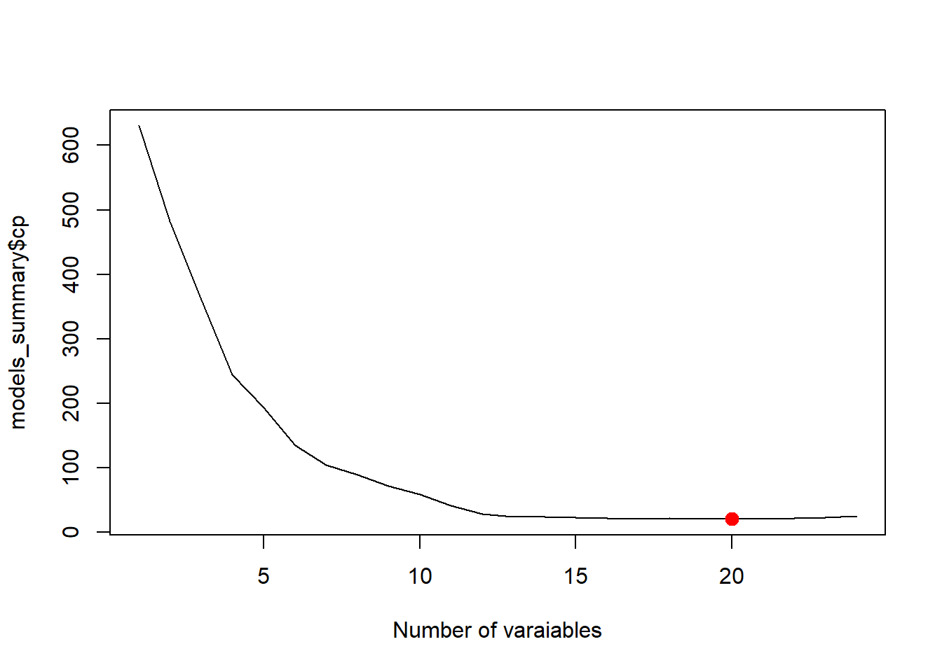
We need to pick 20 variables, and from the table, the variables we need to remove are zn, indus and age. Since rad is a categorical variable represented by multiple dummy variables, all levels must be kept together in the model. Even if some individual coefficients are not significant, we should test the significance of the entire factor using an F-test rather than removing individual levels.

The above selection is the same if we use step.

step(fit_int)
Start:  AIC=-1818.1
log(medv) ~ (crim + zn + indus + chas + nox + rm + age + dis + 
    rad + tax + ptratio + black + lstat) - crim + sqrt(crim) + 
    I(rm^2) + I(lstat^2) + sqrt(crim) * lstat + sqrt(crim) * 
    rm

                   Df Sum of Sq    RSS     AIC
- indus             1   0.01077 12.623 -1819.7
- age               1   0.01259 12.625 -1819.6
- zn                1   0.04912 12.661 -1818.1
<none>                          12.612 -1818.1
- chas              1   0.13887 12.751 -1814.6
- I(rm^2)           1   0.26398 12.876 -1809.6
- black             1   0.34418 12.956 -1806.5
- tax               1   0.43581 13.048 -1802.9
- nox               1   0.45819 13.070 -1802.0
- dis               1   0.70671 13.319 -1792.5
- rm:sqrt(crim)     1   0.71953 13.332 -1792.0
- ptratio           1   0.74902 13.361 -1790.9
- rad               8   1.28103 13.893 -1785.2
- I(lstat^2)        1   1.14346 13.755 -1776.2
- lstat:sqrt(crim)  1   2.28857 14.900 -1735.7

Step:  AIC=-1819.66
log(medv) ~ zn + chas + nox + rm + age + dis + rad + tax + ptratio + 
    black + lstat + sqrt(crim) + I(rm^2) + I(lstat^2) + lstat:sqrt(crim) + 
    rm:sqrt(crim)

                   Df Sum of Sq    RSS     AIC
- age               1   0.01338 12.636 -1821.1
- zn                1   0.04443 12.667 -1819.9
<none>                          12.623 -1819.7
- chas              1   0.14650 12.769 -1815.8
- I(rm^2)           1   0.25855 12.881 -1811.4
- black             1   0.34214 12.965 -1808.1
- nox               1   0.45375 13.076 -1803.8
- tax               1   0.45726 13.080 -1803.7
- rm:sqrt(crim)     1   0.71679 13.339 -1793.7
- ptratio           1   0.74183 13.365 -1792.8
- dis               1   0.77851 13.401 -1791.4
- rad               8   1.31706 13.940 -1785.4
- I(lstat^2)        1   1.17569 13.798 -1776.6
- lstat:sqrt(crim)  1   2.41183 15.035 -1733.2

Step:  AIC=-1821.13
log(medv) ~ zn + chas + nox + rm + dis + rad + tax + ptratio + 
    black + lstat + sqrt(crim) + I(rm^2) + I(lstat^2) + lstat:sqrt(crim) + 
    rm:sqrt(crim)

                   Df Sum of Sq    RSS     AIC
- zn                1   0.04768 12.684 -1821.2
<none>                          12.636 -1821.1
- chas              1   0.14352 12.780 -1817.4
- I(rm^2)           1   0.25693 12.893 -1812.9
- black             1   0.33271 12.969 -1810.0
- tax               1   0.46365 13.100 -1804.9
- nox               1   0.51974 13.156 -1802.7
- rm:sqrt(crim)     1   0.70511 13.341 -1795.7
- ptratio           1   0.77704 13.413 -1792.9
- dis               1   0.78139 13.418 -1792.8
- rad               8   1.37636 14.012 -1784.8
- I(lstat^2)        1   1.24999 13.886 -1775.4
- lstat:sqrt(crim)  1   2.45365 15.090 -1733.3

Step:  AIC=-1821.22
log(medv) ~ chas + nox + rm + dis + rad + tax + ptratio + black + 
    lstat + sqrt(crim) + I(rm^2) + I(lstat^2) + lstat:sqrt(crim) + 
    rm:sqrt(crim)

                   Df Sum of Sq    RSS     AIC
<none>                          12.684 -1821.2
- chas              1   0.14541 12.829 -1817.5
- I(rm^2)           1   0.25115 12.935 -1813.3
- black             1   0.33199 13.016 -1810.2
- tax               1   0.43225 13.116 -1806.3
- nox               1   0.53593 13.220 -1802.3
- rm:sqrt(crim)     1   0.75049 13.434 -1794.1
- dis               1   0.79620 13.480 -1792.4
- rad               8   1.33524 14.019 -1786.6
- ptratio           1   1.01538 13.699 -1784.3
- I(lstat^2)        1   1.30254 13.986 -1773.8
- lstat:sqrt(crim)  1   2.43560 15.119 -1734.3

Call:
lm(formula = log(medv) ~ chas + nox + rm + dis + rad + tax + 
    ptratio + black + lstat + sqrt(crim) + I(rm^2) + I(lstat^2) + 
    lstat:sqrt(crim) + rm:sqrt(crim), data = Boston)

Coefficients:
     (Intercept)             chas1               nox                rm  
       4.5059381         0.0702287        -0.5731773        -0.2238236  
             dis              rad2              rad3              rad4  
      -0.0322959         0.0520156         0.1364592         0.0888065  
            rad5              rad6              rad7              rad8  
       0.1217036         0.1161403         0.1553079         0.1141133  
           rad24               tax           ptratio             black  
       0.3943541        -0.0004944        -0.0297147         0.0003294  
           lstat        sqrt(crim)           I(rm^2)        I(lstat^2)  
      -0.0471656         0.4674652         0.0319646         0.0011399  
lstat:sqrt(crim)     rm:sqrt(crim)  
      -0.0108782        -0.0586671  

We now delete these variables, and get a new model.

fit <- lm(
    log(medv) ~ . - crim - zn - indus - age + sqrt(crim) + I(rm^2) + I(lstat^2) + sqrt(crim) * lstat + sqrt(crim) * rm,
    data = Boston
)

We apply the nested F-test to confirm the deleting.

anova(fit, fit_int)
Analysis of Variance Table

Model 1: log(medv) ~ (crim + zn + indus + chas + nox + rm + age + dis + 
    rad + tax + ptratio + black + lstat) - crim - zn - indus - 
    age + sqrt(crim) + I(rm^2) + I(lstat^2) + sqrt(crim) * lstat + 
    sqrt(crim) * rm
Model 2: log(medv) ~ (crim + zn + indus + chas + nox + rm + age + dis + 
    rad + tax + ptratio + black + lstat) - crim + sqrt(crim) + 
    I(rm^2) + I(lstat^2) + sqrt(crim) * lstat + sqrt(crim) * 
    rm
  Res.Df    RSS Df Sum of Sq      F Pr(>F)
1    484 12.684                           
2    481 12.612  3  0.071827 0.9131 0.4344

It is not significant. Therefore it is safe to remove them. We do a final check up.

summary(fit)

Call:
lm(formula = log(medv) ~ . - crim - zn - indus - age + sqrt(crim) + 
    I(rm^2) + I(lstat^2) + sqrt(crim) * lstat + sqrt(crim) * 
    rm, data = Boston)

Residuals:
     Min       1Q   Median       3Q      Max 
-0.68354 -0.07637 -0.00795  0.08444  0.76250 

Coefficients:
                   Estimate Std. Error t value Pr(>|t|)    
(Intercept)       4.506e+00  5.314e-01   8.480 2.75e-16 ***
chas1             7.023e-02  2.981e-02   2.356 0.018893 *  
nox              -5.732e-01  1.267e-01  -4.522 7.71e-06 ***
rm               -2.238e-01  1.427e-01  -1.568 0.117508    
dis              -3.230e-02  5.859e-03  -5.512 5.78e-08 ***
rad2              5.202e-02  5.047e-02   1.031 0.303246    
rad3              1.365e-01  4.565e-02   2.989 0.002942 ** 
rad4              8.881e-02  4.098e-02   2.167 0.030731 *  
rad5              1.217e-01  4.112e-02   2.960 0.003229 ** 
rad6              1.161e-01  5.017e-02   2.315 0.021025 *  
rad7              1.553e-01  5.399e-02   2.877 0.004195 ** 
rad8              1.141e-01  5.060e-02   2.255 0.024569 *  
rad24             3.944e-01  6.502e-02   6.065 2.65e-09 ***
tax              -4.944e-04  1.217e-04  -4.061 5.69e-05 ***
ptratio          -2.971e-02  4.774e-03  -6.225 1.05e-09 ***
black             3.294e-04  9.254e-05   3.559 0.000409 ***
lstat            -4.717e-02  5.258e-03  -8.970  < 2e-16 ***
sqrt(crim)        4.675e-01  8.062e-02   5.799 1.21e-08 ***
I(rm^2)           3.196e-02  1.033e-02   3.096 0.002077 ** 
I(lstat^2)        1.140e-03  1.617e-04   7.050 6.20e-12 ***
lstat:sqrt(crim) -1.088e-02  1.128e-03  -9.641  < 2e-16 ***
rm:sqrt(crim)    -5.867e-02  1.096e-02  -5.351 1.35e-07 ***
---
Signif. codes:  0 '***' 0.001 '**' 0.01 '*' 0.05 '.' 0.1 ' ' 1

Residual standard error: 0.1619 on 484 degrees of freedom
Multiple R-squared:  0.8497,    Adjusted R-squared:  0.8432 
F-statistic: 130.3 on 21 and 484 DF,  p-value: < 2.2e-16
par(mfrow = c(2, 2))
plot(fit)

par(mfrow = c(1, 1))

14.4 Step 4: Diagnose the Final Model

We can also check multicollinearity and influence numerically.

vif(fit)
there are higher-order terms (interactions) in this model
consider setting type = 'predictor'; see ?vif
                       GVIF Df GVIF^(1/(2*Df))
chas               1.105037  1        1.051207
nox                4.156822  1        2.038829
rm               193.812361  1       13.921651
dis                2.933328  1        1.712696
rad               19.430756  8        1.203734
tax                8.110976  1        2.847978
ptratio            2.058263  1        1.434665
black              1.375484  1        1.172810
lstat             27.171883  1        5.212666
sqrt(crim)       263.762982  1       16.240781
I(rm^2)          169.368441  1       13.014163
I(lstat^2)        28.071285  1        5.298234
lstat:sqrt(crim)  30.127124  1        5.488818
rm:sqrt(crim)    170.122683  1       13.043109

Polynomial and interaction terms often lead to higher VIF values because they are inherently correlated with the variables from which they are constructed. In this model, variables such as rm, lstat, and sqrt(crim) appear together with their squared terms or interaction terms, which naturally induces multicollinearity. This behavior is expected when a variable and its polynomial, transformed, or interaction terms are included in the model. Therefore, moderately large VIF values in this situation do not necessarily indicate a problem and are not, by themselves, a reason to remove these terms.

rs <- rstudent(fit)
cd <- cooks.distance(fit)
lev <- hatvalues(fit)
nr <- nrow(Boston)

c(
    max_abs_studentized = max(abs(rs)),
    num_abs_studentized_gt_3 = sum(abs(rs) > 3),
    num_cooks_gt_4_over_n = sum(cd > 4 / nr),
    num_high_leverage = sum(lev > 2 * length(coef(fit)) / nr)
)
     max_abs_studentized num_abs_studentized_gt_3    num_cooks_gt_4_over_n 
                4.914443                12.000000                31.000000 
       num_high_leverage 
               30.000000 

The diagnostics show that

  • the largest absolute studentized residual is about \(4.9\),
  • 12 observations exceeding the rule-of-thumb threshold of \(3\),
  • about \(31\) observations have Cook’s distance greater than \(4/n\),
  • roughly 30 observations exceed the \(2p/n\).

These values indicate the presence of some unusual observations, which is not surprising for a dataset of this size and with a model containing several nonlinear and interaction terms. However,

  • none of the observations appear to be extremely influential.

Unless these observations correspond to data entry or measurement errors, it is generally preferable to keep them in the analysis and simply report their presence.

To improve interpretability and reduce VIF values, we may center some of the variables. The vif output shows relatively large values for sqrt(crim), rm, lstat, and their associated polynomial and interaction terms. This occurs because such terms are naturally correlated with the variables from which they are constructed. Therefore we center these variables before forming the polynomial and interaction terms.

Note that centering is not required for statistical correctness. It does not change the fitted values or overall model fit, but it can reduce VIF values and make the coefficients easier to interpret.

Boston$sqrt_crim <- sqrt(Boston$crim)

Boston$sqrt_crim_c <- scale(Boston$sqrt_crim, scale = FALSE)
Boston$rm_c <- scale(Boston$rm, scale = FALSE)
Boston$lstat_c <- scale(Boston$lstat, scale = FALSE)

fit_final <- lm(
    log(medv) ~ chas + nox + dis + rad + tax + ptratio + black +
        sqrt_crim_c + rm_c + lstat_c +
        I(rm_c^2) + I(lstat_c^2) +
        sqrt_crim_c:lstat_c + sqrt_crim_c:rm_c,
    data = Boston
)
vif(fit_final)
there are higher-order terms (interactions) in this model
consider setting type = 'predictor'; see ?vif
                         GVIF Df GVIF^(1/(2*Df))
chas                 1.105037  1        1.051207
nox                  4.156822  1        2.038829
dis                  2.933328  1        1.712696
rad                 19.430756  8        1.203734
tax                  8.110976  1        2.847978
ptratio              2.058263  1        1.434665
black                1.375484  1        1.172810
sqrt_crim_c          7.371623  1        2.715073
rm_c                 2.404949  1        1.550790
lstat_c              4.452527  1        2.110101
I(rm_c^2)            1.929409  1        1.389032
I(lstat_c^2)         3.237789  1        1.799386
sqrt_crim_c:lstat_c  4.683008  1        2.164026
sqrt_crim_c:rm_c     3.046427  1        1.745402
summary(fit_final)

Call:
lm(formula = log(medv) ~ chas + nox + dis + rad + tax + ptratio + 
    black + sqrt_crim_c + rm_c + lstat_c + I(rm_c^2) + I(lstat_c^2) + 
    sqrt_crim_c:lstat_c + sqrt_crim_c:rm_c, data = Boston)

Residuals:
     Min       1Q   Median       3Q      Max 
-0.68354 -0.07637 -0.00795  0.08444  0.76250 

Coefficients:
                      Estimate Std. Error t value Pr(>|t|)    
(Intercept)          3.900e+00  1.447e-01  26.956  < 2e-16 ***
chas1                7.023e-02  2.981e-02   2.356 0.018893 *  
nox                 -5.732e-01  1.267e-01  -4.522 7.71e-06 ***
dis                 -3.230e-02  5.859e-03  -5.512 5.78e-08 ***
rad2                 5.202e-02  5.047e-02   1.031 0.303246    
rad3                 1.365e-01  4.565e-02   2.989 0.002942 ** 
rad4                 8.881e-02  4.098e-02   2.167 0.030731 *  
rad5                 1.217e-01  4.112e-02   2.960 0.003229 ** 
rad6                 1.161e-01  5.017e-02   2.315 0.021025 *  
rad7                 1.553e-01  5.399e-02   2.877 0.004195 ** 
rad8                 1.141e-01  5.060e-02   2.255 0.024569 *  
rad24                3.944e-01  6.502e-02   6.065 2.65e-09 ***
tax                 -4.944e-04  1.217e-04  -4.061 5.69e-05 ***
ptratio             -2.971e-02  4.774e-03  -6.225 1.05e-09 ***
black                3.294e-04  9.254e-05   3.559 0.000409 ***
sqrt_crim_c         -3.888e-02  1.348e-02  -2.885 0.004091 ** 
rm_c                 1.058e-01  1.590e-02   6.655 7.67e-11 ***
lstat_c             -3.169e-02  2.129e-03 -14.890  < 2e-16 ***
I(rm_c^2)            3.196e-02  1.033e-02   3.096 0.002077 ** 
I(lstat_c^2)         1.140e-03  1.617e-04   7.050 6.20e-12 ***
sqrt_crim_c:lstat_c -1.088e-02  1.128e-03  -9.641  < 2e-16 ***
sqrt_crim_c:rm_c    -5.867e-02  1.096e-02  -5.351 1.35e-07 ***
---
Signif. codes:  0 '***' 0.001 '**' 0.01 '*' 0.05 '.' 0.1 ' ' 1

Residual standard error: 0.1619 on 484 degrees of freedom
Multiple R-squared:  0.8497,    Adjusted R-squared:  0.8432 
F-statistic: 130.3 on 21 and 484 DF,  p-value: < 2.2e-16

Now we return to the standard diagnostics for the refined model.

par(mfrow = c(2, 2))
plot(fit_final)
par(mfrow = c(1, 1))

These plots are substantially improved compared with those from the original untransformed model:

  • The residuals versus fitted plot shows no strong systematic pattern, indicating that the nonlinear terms have largely captured the curvature present in the original model.
  • The spread of the residuals is more stable across fitted values, although a mild heteroscedastic pattern may still remain.
  • The Q–Q plot follows the reference line reasonably well in the center but shows deviations in the tails, indicating mild departures from normality.
  • The Scale–Location plot suggests that the variance is more stable than in the original model, although a mild heteroscedastic pattern may still remain.
  • The residuals versus leverage plot shows several observations with moderate leverage, but none appear to have extremely large Cook’s distance values.

Overall, the diagnostic plots suggest that the refined model satisfies the regression assumptions much better than the original additive model.

14.5 Final Model

Our final working model is

\[ \begin{split} \log(\texttt{medv}) = &\beta_0 + \beta_1\texttt{chas}+ \beta_2\texttt{nox} + \beta_3\texttt{dis} + \beta_4\texttt{rad} + \beta_5\texttt{tax} + \beta_6\texttt{ptratio}+ \beta_7\texttt{black}+\beta_8\sqrt{\texttt{crim}}\\ +&\beta_9\texttt{rm}+ \beta_{10}\texttt{lstat}+ \beta_{11}\texttt{rm}^2+ \beta_{12}\texttt{lstat}^2+\beta_{13}\texttt{lstat}\cdot\sqrt{\texttt{crim}} +\beta_{14}\texttt{rm}\cdot\sqrt{\texttt{crim}}+ \varepsilon. \end{split} \]

In R formula form, this is:

formula(fit_final)
log(medv) ~ chas + nox + dis + rad + tax + ptratio + black + 
    sqrt_crim_c + rm_c + lstat_c + I(rm_c^2) + I(lstat_c^2) + 
    sqrt_crim_c:lstat_c + sqrt_crim_c:rm_c

The main conclusions are:

  • Transforming the response using log(medv) is supported by the Box–Cox analysis and helps stabilize the variance.
  • Adding quadratic, interaction, and transformed terms captures nonlinear patterns that the simple additive linear model cannot represent.
  • The final model explains about 85% of the variation in log(medv), with an adjusted \(R^2_{adj}\) around \(0.84\). The residual standard error is \(0.1619\).