The Boston housing dataset originates from a hedonic price analysis of 506 census tracts in the Boston Standard Metropolitan Statistical Area conducted by Harrison and Rubinfeld to estimate households’ willingness to pay for improvements in air quality, particularly reductions in nitrogen oxides (NOx) concentrations [1]. The data were assembled primarily from 1970 U.S. Census housing tabulations combined with modeled environmental pollution measures. Since its original publication, the dataset has been widely disseminated as the Boston dataset in econometrics, statistics, and machine learning, where it is commonly used to illustrate and evaluate linear regression methods. It was notably employed by Belsley, Kuh, and Welsch in Regression Diagnostics: Identifying Influential Data and Sources of Collinearity (pp. 244–261) [2] to demonstrate diagnostic techniques for detecting influential observations and multicollinearity, and has subsequently appeared in numerous methodological studies, including Quinlan’s work on combining instance-based and model-based learning [3].
In R, the MASS library contains Boston data set, which has 506 rows and 14 columns. The dataset records medv (median house value) and 13 predictors for 506 neighborhoods around Boston.
7.2 Explore the Boston Housing Dataset
First of all, let’s take a look at the variables in the dataset Boston.
head() — print out the first 5 rows of the dataset;
dim() — print out the shape of the dataset.
You may use ?Boston to look at the brief describption.
Since we would like to directly work with varibles in the dataset, it is better to attach it to the working space.
attach(Boston)
7.2.1 Data Type
First we need to know the data type of every variable. Based on the information we have, we know
Variable
Description
Type
crim
Per capita crime rate by town
Numerical, continuous
zn
Proportion of residential land zoned for lots over 25,000 sq.ft.
Numerical, continuous
indus
Proportion of non-retail business acres per town
Numerical, continuous
chas
Charles River dummy variable (1 if tract bounds river; 0 otherwise)
Categorical, nominal
nox
Nitrogen oxides concentration (parts per 10 million)
Numerical, continuous
rm
Average number of rooms per dwelling
Numerical, continuous
age
Proportion of owner-occupied units built prior to 1940
Numerical, continuous
dis
Weighted mean distance to five Boston employment centers
Numerical, continuous
rad
Index of accessibility to radial highways (larger = better accessibility)
Categorical, ordinal
tax
Full-value property-tax rate per $10,000
Numerical, continuous
ptratio
Pupil–teacher ratio by town
Numerical, continuous
black
\(1000(B_k - 0.63)^2\), where \(B_k\) is the proportion of Black residents
Numerical, continuous
lstat
Percentage of lower-status population
Numerical, continuous
medv
Median value of owner-occupied homes (in $1,000s)
Numerical, continuous
7.2.2 Summary of all the variables
Usually we would like to check two things: the distribution of each variable, and finding all missing values.
Are there any missing values?
sapply(Boston, anyNA)
   crim      zn   indus    chas     nox      rm     age     dis     rad     tax
  FALSE   FALSE   FALSE   FALSE   FALSE   FALSE   FALSE   FALSE   FALSE   FALSE
ptratio   black   lstat    medv
  FALSE   FALSE   FALSE   FALSE
From the output, we know there is no missing values in the Boston dataset.
Next, we find the summary of all the 13 variables as follows. These summary shows a brief glance of the distributions of all variables.
summary(Boston)
      crim                zn             indus            chas
 Min.   : 0.00632   Min.   :  0.00   Min.   : 0.46   Min.   :0.00000
 1st Qu.: 0.08205   1st Qu.:  0.00   1st Qu.: 5.19   1st Qu.:0.00000
 Median : 0.25651   Median :  0.00   Median : 9.69   Median :0.00000
 Mean   : 3.61352   Mean   : 11.36   Mean   :11.14   Mean   :0.06917
 3rd Qu.: 3.67708   3rd Qu.: 12.50   3rd Qu.:18.10   3rd Qu.:0.00000
 Max.   :88.97620   Max.   :100.00   Max.   :27.74   Max.   :1.00000
      nox               rm             age              dis
 Min.   :0.3850   Min.   :3.561   Min.   :  2.90   Min.   : 1.130
 1st Qu.:0.4490   1st Qu.:5.886   1st Qu.: 45.02   1st Qu.: 2.100
 Median :0.5380   Median :6.208   Median : 77.50   Median : 3.207
 Mean   :0.5547   Mean   :6.285   Mean   : 68.57   Mean   : 3.795
 3rd Qu.:0.6240   3rd Qu.:6.623   3rd Qu.: 94.08   3rd Qu.: 5.188
 Max.   :0.8710   Max.   :8.780   Max.   :100.00   Max.   :12.127
      rad              tax           ptratio          black
 Min.   : 1.000   Min.   :187.0   Min.   :12.60   Min.   :  0.32
 1st Qu.: 4.000   1st Qu.:279.0   1st Qu.:17.40   1st Qu.:375.38
 Median : 5.000   Median :330.0   Median :19.05   Median :391.44
 Mean   : 9.549   Mean   :408.2   Mean   :18.46   Mean   :356.67
 3rd Qu.:24.000   3rd Qu.:666.0   3rd Qu.:20.20   3rd Qu.:396.23
 Max.   :24.000   Max.   :711.0   Max.   :22.00   Max.   :396.90
     lstat            medv
 Min.   : 1.73   Min.   : 5.00
 1st Qu.: 6.95   1st Qu.:17.02
 Median :11.36   Median :21.20
 Mean   :12.65   Mean   :22.53
 3rd Qu.:16.95   3rd Qu.:25.00
 Max.   :37.97   Max.   :50.00
Note that chas and rad are supposed to be categorical data. In this summary they are still treated as numerical. Therefore we could change their type if necessary.
      crim                zn             indus            chas
 Min.   : 0.00632   Min.   :  0.00   Min.   : 0.46   Min.   :0.00000
 1st Qu.: 0.08205   1st Qu.:  0.00   1st Qu.: 5.19   1st Qu.:0.00000
 Median : 0.25651   Median :  0.00   Median : 9.69   Median :0.00000
 Mean   : 3.61352   Mean   : 11.36   Mean   :11.14   Mean   :0.06917
 3rd Qu.: 3.67708   3rd Qu.: 12.50   3rd Qu.:18.10   3rd Qu.:0.00000
 Max.   :88.97620   Max.   :100.00   Max.   :27.74   Max.   :1.00000
      nox               rm             age              dis
 Min.   :0.3850   Min.   :3.561   Min.   :  2.90   Min.   : 1.130
 1st Qu.:0.4490   1st Qu.:5.886   1st Qu.: 45.02   1st Qu.: 2.100
 Median :0.5380   Median :6.208   Median : 77.50   Median : 3.207
 Mean   :0.5547   Mean   :6.285   Mean   : 68.57   Mean   : 3.795
 3rd Qu.:0.6240   3rd Qu.:6.623   3rd Qu.: 94.08   3rd Qu.: 5.188
 Max.   :0.8710   Max.   :8.780   Max.   :100.00   Max.   :12.127
      rad              tax           ptratio          black
 Min.   : 1.000   Min.   :187.0   Min.   :12.60   Min.   :  0.32
 1st Qu.: 4.000   1st Qu.:279.0   1st Qu.:17.40   1st Qu.:375.38
 Median : 5.000   Median :330.0   Median :19.05   Median :391.44
 Mean   : 9.549   Mean   :408.2   Mean   :18.46   Mean   :356.67
 3rd Qu.:24.000   3rd Qu.:666.0   3rd Qu.:20.20   3rd Qu.:396.23
 Max.   :24.000   Max.   :711.0   Max.   :22.00   Max.   :396.90
     lstat            medv
 Min.   : 1.73   Min.   : 5.00
 1st Qu.: 6.95   1st Qu.:17.02
 Median :11.36   Median :21.20
 Mean   :12.65   Mean   :22.53
 3rd Qu.:16.95   3rd Qu.:25.00
 Max.   :37.97   Max.   :50.00
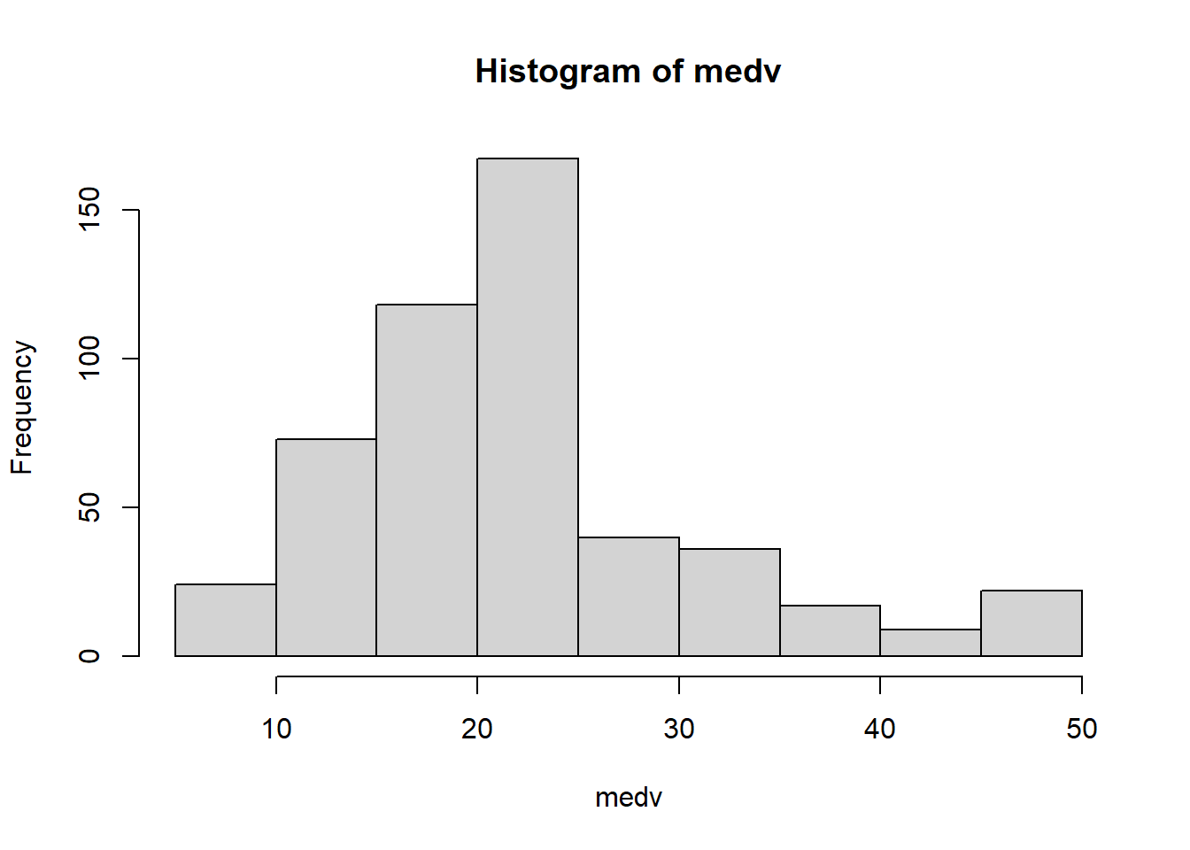
7.2.3 Histogram
We could draw histogram for a particular variable, say medv.
hist(medv)
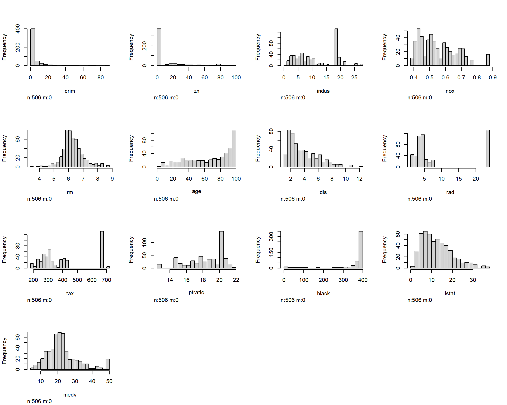
We could also draw all the histogram for all numerical variables in the data frame Boston with the help of `Hmisc::hist.data.frame. Note that categorical data are automatically removed.
library(Hmisc)hist.data.frame(Boston)
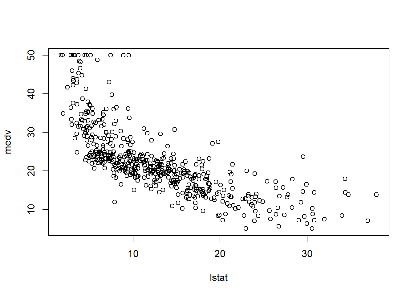
7.2.4 Scatter plot
Finally, the most import plot for regression should be the scatter plot. For example, let us see the relation between lstat and medv.
plot(lstat, medv)
7.3 Simple Linear Regression
We will seek to predict medv using 13 predictors such as rm (average number of rooms per house), age (proportion of the owner-occupied units built prior to 1940), or lstat (percent of households with low socioeconomic status).
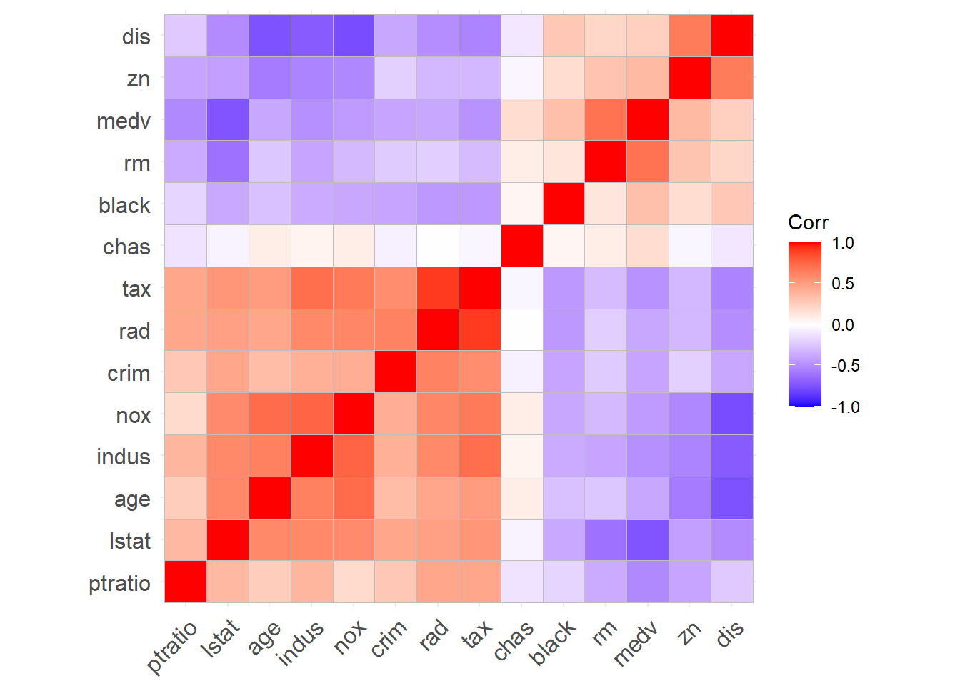
7.3.1 Find a strongest linear correlation
In general there has to be a more complicated analysis about choosing the best variable. In this case in order to demonstrate the idea, we will only use the most correlted numerical variable.
Here, we use corrlation matrix to find the independent variable which has the strongest linear correlation to the dependent variable.
Then we compute the corrlation matrix. We would like to find the column that is most correlated to medv. We find that lstat and medv has the strongest linear correlation.
For the next step, we will explore the linear relationship between the two variables. That is, \(y\)=medv, \(x\)=lstat.
plot(lstat, medv)
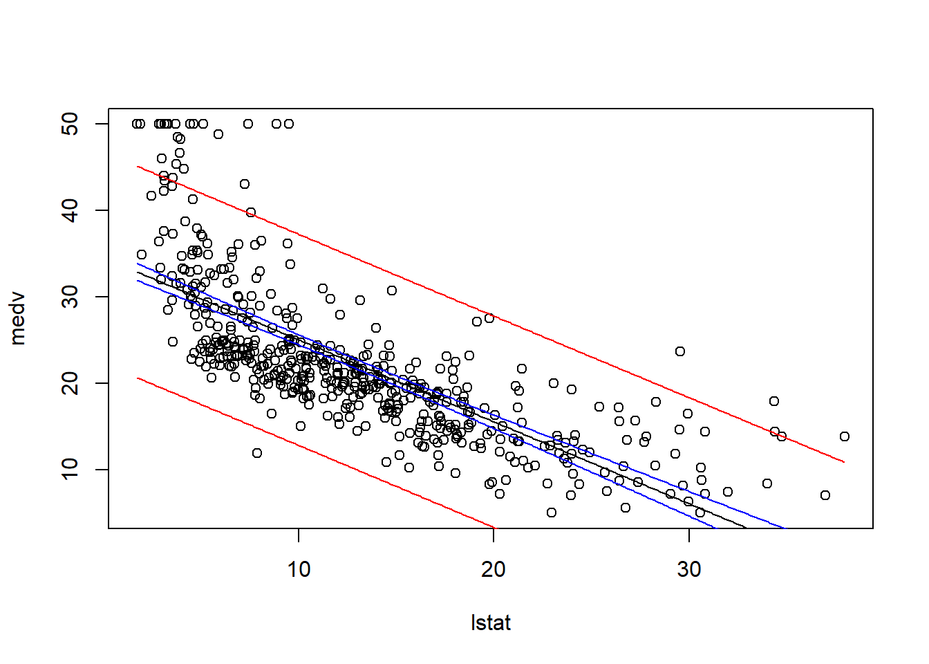
The data appears to demostrate a straight-line relationshiop. As the percentage of lower status of the population (lstat) increase, the median home value decrease, which fits with common sense. The scatterplot shows curvilinear relation, which suggests a curivilinear model might be a better fit. In this chapter, we fit the straight-line model using lm.
The estimated regression equation by using least squares method is \(\hat{y}\)=34.5538409\(+\)(-0.9500494)\(x\).
7.3.2 Test of model utility
We would like to see the output of the model.
anova_alt(model)
Analysis of Variance Table

        Df    SS      MS      F          P
Source   1 23244 23243.9 601.62 5.0811e-88
Error  504 19472    38.6
Total  505 42716
summary(model)
Call:
lm(formula = medv ~ lstat, data = Boston)

Residuals:
    Min      1Q  Median      3Q     Max
-15.168  -3.990  -1.318   2.034  24.500

Coefficients:
            Estimate Std. Error t value Pr(>|t|)
(Intercept) 34.55384    0.56263   61.41   <2e-16 ***
lstat       -0.95005    0.03873  -24.53   <2e-16 ***
---
Signif. codes:  0 '***' 0.001 '**' 0.01 '*' 0.05 '.' 0.1 ' ' 1

Residual standard error: 6.216 on 504 degrees of freedom
Multiple R-squared:  0.5441,    Adjusted R-squared:  0.5432
F-statistic: 601.6 on 1 and 504 DF,  p-value: < 2.2e-16
Let us check the confidence interval for \(\beta_1\).
# Combine to display the coef and confidence interval for the parameters together;coef <-coefficients(summary(model))coef_CI <-confint(model, level =0.95)cbind(coef, coef_CI)
Significance: We test the \(H_0:\beta_1=0\) vs \(H_a: \beta_1\neq 0\). For simple linear regression, the result would be the same as the correlation hypothesis test above. We will conclude percentage of lower status (lstat) is a significant predictor to the median house price (medv).
CI for \(\beta_1\): The confidence interval for slope \(\beta_1\) is (-1.0261482, -0.8739505). We are 95% confident that the mean median home price decreases around 0.874 to 1.026 thousands of dollors per additional percent increase in low-status of the population.
sd for \(\beta_1\): The estimated standard deviation of \(\varepsilon\) is \(s\)=6.2157604, which implies that most of the observed median home price will fall within in approximately \(2s\)=12.4 thousands of dollars of their respective predicted values when using the least squares line.
\(R^2\): The coefficient of determination is 0.544. This value implies that about 54% of the sample variation in median home price is explained by the low-status percent and the median home price. However, as we note that \(R^2\) is not very high, we need to modify our model in the future.
Prediction: With relatively small \(2s\), significant linear relationship between lstat and medv, we could get confidence interval and prediction interval as follows.
plot(lstat, medv)newx <-data.frame(lstat =seq(min(lstat), max(lstat), by =0.1))pred.int <-predict(model, newx, interval ="prediction")conf.int <-predict(model, newx, interval ="confidence")lines(newx$lstat, pred.int[, "fit"])lines(newx$lstat, pred.int[, "lwr"], col ="red")lines(newx$lstat, pred.int[, "upr"], col ="red")lines(newx$lstat, conf.int[, "lwr"], col ="blue")lines(newx$lstat, conf.int[, "upr"], col ="blue")
7.3.3 Residual Analysis
The detailed residual analysis will be covered in the future. Here we only show the very basic analysis, that is the plot of the residual vs the fitted value.
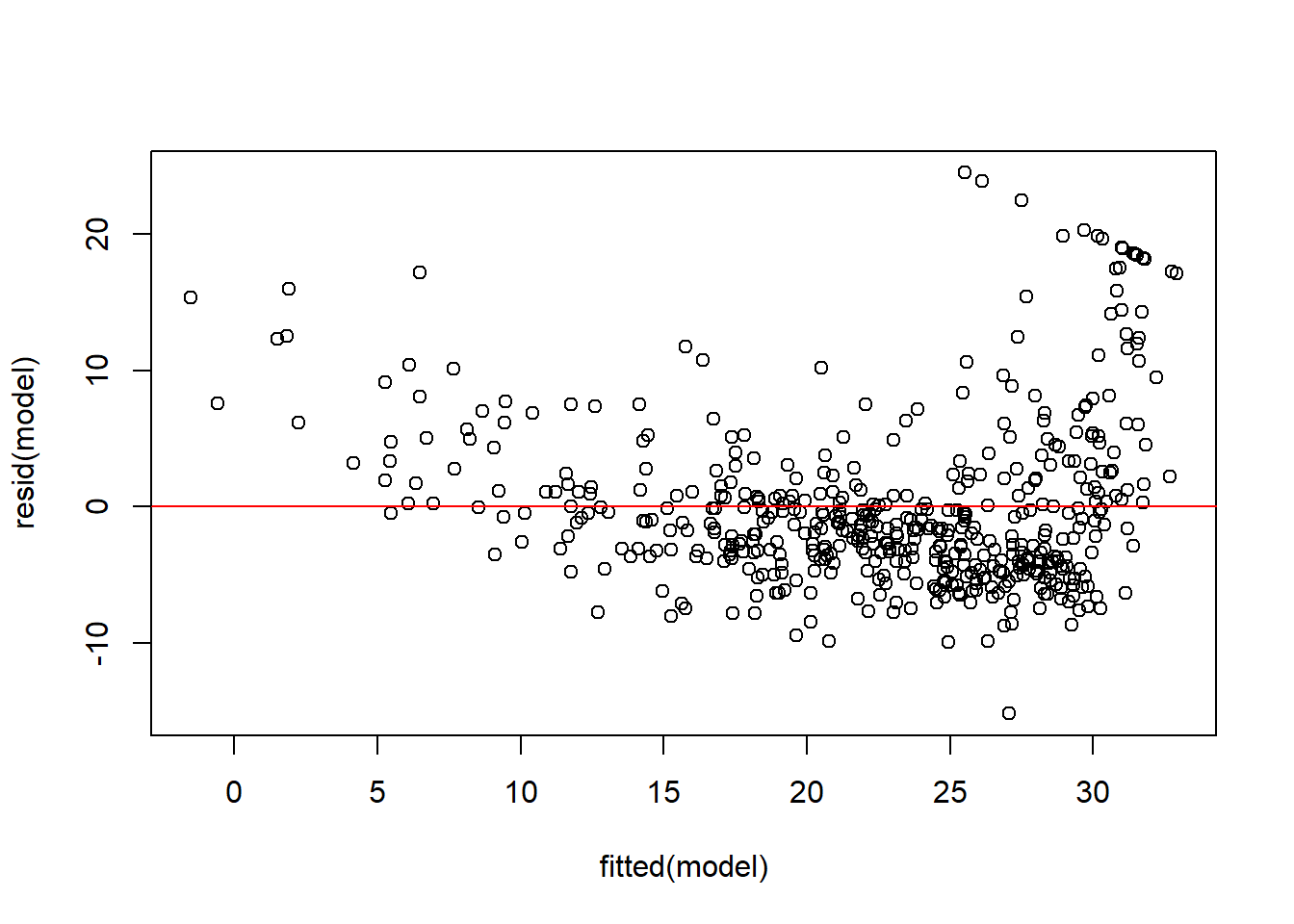
plot(fitted(model), resid(model))abline(h =0, col ="red")
Figure 7.1: Residual plot for the SLR model
We could find that there is a clear u-shape in the residual plot. And the variance shows non-constant variance issue, as the size of the residuals decreases as the value of lstat increase. This residual plot indicates that a multiplicative model may be appropriate.
Belsley, D. A., Kuh, E. and Welsch, R. E. (1980). Regression diagnostics: Identifying influential data and sources of collinearity. John Wiley & Sons, New York.
[3]
Quinlan, J. R. (1993). Combining instance-based and model-based learning. In Proceedings of the tenth international conference on machine learning pp 236–43. Morgan Kaufmann, Amherst, Massachusetts.