2.3. k-NN Project 2: Dating Classification

The data can be downloaded from here.

2.3.1. Background

Helen dated several people and rated them using a three-point scale: 3 is best and 1 is worst. She also collected data from all her dates and recorded them in the file attached. These data contains 3 features:

• Number of frequent flyer miles earned per year

• Percentage of time spent playing video games

• Liters of ice cream consumed per week

We would like to predict her ratings of new dates when we are given the three features.

The data contains four columns, while the first column refers to Mileage, the second Gamingtime, the third Icecream and the fourth Rating.

2.3.2. Look at Data

We first load the data and store it into a DataFrame.

import numpy as np
import pandas as pd
import matplotlib.pyplot as plt

df = pd.read_csv('./assests/datasets/datingTestSet2.txt', sep='\t', header=None)
df.head()

	0	1	2	3
0	40920	8.326976	0.953952	3
1	14488	7.153469	1.673904	2
2	26052	1.441871	0.805124	1
3	75136	13.147394	0.428964	1
4	38344	1.669788	0.134296	1

To make it easier to read, we would like to change the name of the columns.

df = df.rename(columns={0: "Mileage", 1: "Gamingtime", 2: 'Icecream', 3: 'Rating'})
df.head()

	Mileage	Gamingtime	Icecream	Rating
0	40920	8.326976	0.953952	3
1	14488	7.153469	1.673904	2
2	26052	1.441871	0.805124	1
3	75136	13.147394	0.428964	1
4	38344	1.669788	0.134296	1

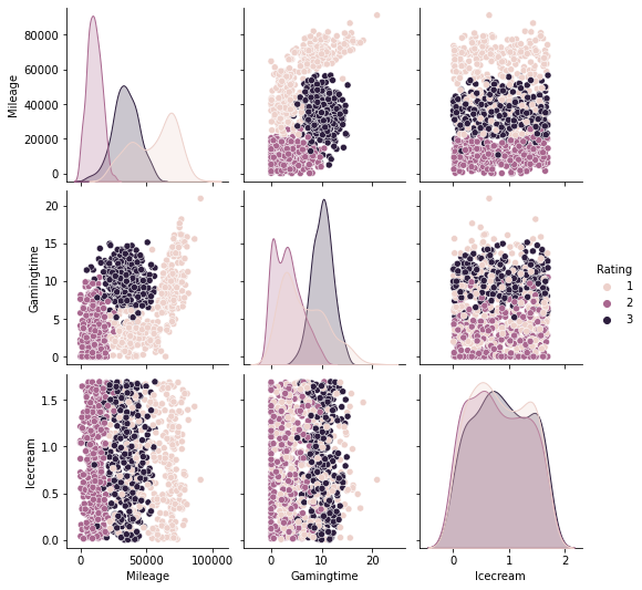
Since now we have more than 2 features, it is not suitable to directly draw scatter plots. We use seaborn.pairplot to look at the pairplot. From the below plots, before we apply any tricks, it seems that Milegae and Gamingtime are better than Icecream to classify the data points.

import seaborn as sns
sns.pairplot(data=df, hue='Rating')

<seaborn.axisgrid.PairGrid at 0x1af8d4881c0>

2.3.3. Applying kNN

Similar to the previous example, we will apply both methods for comparisons.

from sklearn.model_selection import train_test_split
from assests.codes.knn import encodeNorm
X = np.array(df[['Mileage', 'Gamingtime', 'Icecream']])
y = np.array(df['Rating'])

X_train, X_test, y_train, y_test = train_test_split(X, y, test_size=0.1, random_state=40, stratify=y)

X_train_norm, parameters = encodeNorm(X_train)
X_test_norm, _ = encodeNorm(X_test, parameters=parameters)

# Using our codes.
from assests.codes.knn import classify_kNN

n_neighbors = 10
y_pred = np.array([classify_kNN(row, X_train_norm, y_train, k=n_neighbors)
                   for row in X_test_norm])

acc = np.mean(y_pred == y_test)
print(acc)

0.93

# Using sklearn.
from sklearn.pipeline import Pipeline
from sklearn.preprocessing import MinMaxScaler
from sklearn.neighbors import KNeighborsClassifier
from sklearn.metrics import accuracy_score

steps = [('scaler', MinMaxScaler()),
         ('knn', KNeighborsClassifier(n_neighbors, weights="uniform",
                                      metric="euclidean", algorithm='brute'))]
pipe = Pipeline(steps=steps)
pipe.fit(X_train, y_train)
y_pipe = pipe.predict(X_test)
print(accuracy_score(y_pipe, y_test))

0.93

2.3.4. Choosing k Value

Similar to the previous section, we can run tests on k value to choose one to be used in our model using GridSearchCV.

from sklearn.model_selection import GridSearchCV, cross_val_score
n_list = list(range(1, 101))
parameters = dict(knn__n_neighbors=n_list)
clf = GridSearchCV(pipe, parameters)
clf.fit(X, y)
print(clf.best_estimator_.get_params()["knn__n_neighbors"])

4

From this result, in this case the best k is 4. The corresponding cross-validation score is computed below.

cv_scores = cross_val_score(clf.best_estimator_, X, y, cv=5)
print(np.mean(cv_scores))

0.952